Machine Learning Algorithms From Scratch: Logistic Regression

Introduction
Logistic regression is a classification algorithm used to assign observations to a discrete set of classes. Unlike linear regression which outputs continuous number values, logistic regression transforms its output using the logistic sigmoid function to return a probability value which can then be mapped to two or more discrete classes.
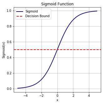
In order to map predicted values to probabilities, we use the sigmoid function. The function maps any real value into another value between 0 and 1. In machine learning, we use sigmoid to map predictions to probabilities.
Sigmoid Function: $f(x) = \frac{1}{1 + exp(-x)}$
# loading libraries
import numpy as np
import matplotlib.pyplot as plt
import matplotlib as mpl
import seaborn as sns

from IPython.core.display import display, HTML
import warnings

sns.set_style("ticks")
mpl.rcParams["axes.linewidth"] = 2
mpl.rcParams["lines.linewidth"] = 2
warnings.filterwarnings("ignore")
display(HTML("<style>.container { width:95% !important; }</style>"))


def sigmoid(x):
    """
    Returns sigmoid(x)
    """
    return 1.0/(1 + np.exp(-x))

def plot_sigmoid(x):
    """
    Plots sigmoid(x)
    """
    fig, ax = plt.subplots(figsize=(5,5))
    ax.plot(x, sigmoid(x), lw=2, c="navy", label="Sigmoid")
    ax.axhline(0.5, lw=2, ls="--", c="red", label="Decision Bound")
    ax.set(title="Sigmoid Function",
           xlabel="x",
           ylabel="Sigmoid(x)")
    ax.grid(True)
    ax.legend(loc=0)
    plt.plot()
# define x to plot sigmoid(x)
x = np.linspace(-5, 5, 100)
plot_sigmoid(x)
The main algorithm to develop Logistic Regression is based on updating weights using Gradient Descent approach iteratively.
- Define linear model: $z = wx + b$
- Define prediction: $\hat{y} = sigmoid(z) = sigmoid(wx + b) = \frac{1}{1 + \exp({-(wx+b)})}$
- Update weights: $w = w - lr \times dw$ where $dw = \frac{1}{N} \Sigma_{i=1}^{N}(2x_i(\hat{y_i} - y_i))$
- Update bias $b = b - lr \times db$ where $db = \frac{1}{N} \Sigma_{i=1}^{N}(\hat{y_i} - y_i)$
class LogisticRegression:
    """
    Logistic Regression based on Gradient Descent
    z = wx + b
    y_hat = sigmoid(z) = sigmoid(wx + b) = 1/(1 + exp[-(wx+b)])
    update rules: w = w - lr * dw
                  b = b - lr * db
    where dw = 1/N sum(2x(y_hat - y))
          db = 1/N sum(2(y_hat - y))
    Parameters
    ----------
    lr: float, optional (default=0.001)
        Learning rate used of updating weights/bias
    n_iters: int, optional (default=1000)
        Maximum number of iterations to update weights/bias
    weights: numpy.array, optional (default=None)
        Weights array of shape (n_features, ) where
        will be initialized as zeros
    bias: float, optional (default=None)
        Bias value where will be initialized as zero
    """

    def __init__(self, learning_rate=0.001, n_iters=1000, weights=None, bias=None):
        self.learning_rate = learning_rate
        self.n_iters = n_iters
        self.weights = None
        self.bias = None

    def fit(self, X_train, y_train):
        """
        Train model using iterative gradient descent
        Parameters
        ----------
        X_train: numpy.array
            Training feature matrix
        y_train: 1D numpy.array or list
            Training binary class labels [0, 1]
        """
        # unpack the shape of X_train
        n_samples, n_features = X_train.shape

        # initialize weights and bias with zeros
        self.weights = np.zeros(n_features)
        self.bias = 0.0

        # main loop
        # self.loss = []
        for _ in range(self.n_iters):
            z = np.dot(X_train, self.weights) + self.bias
            y_hat = self._sigmoid(z)

            # update weights + bias
            dw = (1.0 / n_samples) * 2 * np.dot(X_train.T, (y_hat - y_train))
            db = (1.0 / n_samples) * 2 * np.sum(y_hat - y_train)

            self.weights -= self.learning_rate * dw
            self.bias -= self.learning_rate * db

        return None

    def predict_proba(self, X_test):
        """
        Prediction probability of the test samples
        Parameters
        ----------
        X_test: numpy.array
            Testing feature matrix
        """
        z = np.dot(X_test, self.weights) + self.bias
        y_pred_proba = self._sigmoid(z)

        return y_pred_proba

    def predict(self, X_test, threshold=0.5):
        """
        Prediction class of the test samples
        Parameters
        ----------
        X_test: numpy.array
            Testing feature matrix
        threshold: float, optional (default=0.5)
            Threshold to define predicted classes
        """
        y_pred_proba = self.predict_proba(X_test)
        y_pred = [1 if x >= threshold else 0 for x in y_pred_proba]

        return y_pred

    def plot_decision_boundary(self, X_test, y_test, threshold=0.5, figsize=(8, 6)):
        """
        Plot the decision boundary
        Parameters
        ----------
        X_test: numpy.array
            Testing feature matrix
        y_test: 1D numpy.array or list
            Testing targets
        threshold: float, optional (default=0.5)
            Threshold to define predicted classes
        figsize: tuple, optional (default=(8,6))
            Figure size
        """
        # calc pred_proba
        y_pred_proba = self.predict_proba(X_test)

        # define positive and negative classes
        pos_class = []
        neg_class = []
        for i in range(len(y_pred_proba)):
            if y_test[i] == 1:
                pos_class.append(y_pred_proba[i])
            else:
                neg_class.append(y_pred_proba[i])

        # plotting
        fig, ax = plt.subplots(figsize=figsize)
        ax.scatter(
            range(len(pos_class)),
            pos_class,
            s=25,
            color="navy",
            marker="o",
            label="Positive Class",
        )
        ax.scatter(
            range(len(neg_class)),
            neg_class,
            s=25,
            color="red",
            marker="s",
            label="Negative Class",
        )
        ax.axhline(
            threshold,
            lw=2,
            ls="--",
            color="black",
            label=f"Decision Bound = {threshold}",
        )
        ax.set_title("Decision Boundary")
        ax.set_xlabel("# of Samples", fontsize=12)
        ax.set_ylabel("Predicted Probability", fontsize=12)
        ax.tick_params(axis="both", which="major", labelsize=12)
        ax.legend(bbox_to_anchor=(1.2, 0.5), loc="center", ncol=1, framealpha=0.0)
        plt.show()

    def _sigmoid(self, z):
        """
        Sigmoid Function
        f(z) = 1/(1 + exp(-z))
        """

        return 1.0 / (1 + np.exp(-z))
This is part of the ML-Algs library which can be downloaded via PIP or from Git.
# you can simply do
!pip install mlalgs
# or cloning the project directly from GitHub
!git clone https://github.com/amirhessam88/ml-algs.git

# change directory to the project
%cd ml-algs

# installing requirements
!pip install -r requirements.txt
# loading libraries
from mlalgs.logistic_regression import LogisticRegression
from sklearn import datasets
from sklearn.model_selection import train_test_split
from sklearn.metrics import accuracy_score
Sample breast cancer data for binary classification task. I have used stratifed train/test splits where test size is the 20\% of the data.
# loading data
data = datasets.load_breast_cancer()
X, y = data.data, data.target
X_train, X_test, y_train, y_test = train_test_split(X, y,
                                                    test_size=0.2,
                                                    shuffle=True,
                                                    random_state=1367,
                                                    stratify=y)
Now, train the model using our algorithm.
# define model
clf = LogisticRegression()
# train model
clf.fit(X_train, y_train)
# predicted class
y_pred = clf.predict(X_test)
# predicted proba
y_pred_proba = clf.predict_proba(X_test)
# accuracy
accuracy_score(y_test, y_pred)
0.9298245614035088
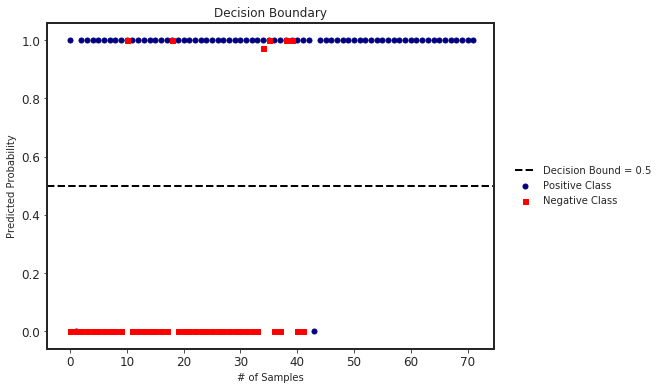
We can also plot the decision boundary and the predicted probabilities in each class.
clf.plot_decision_boundary(X_test, y_test)
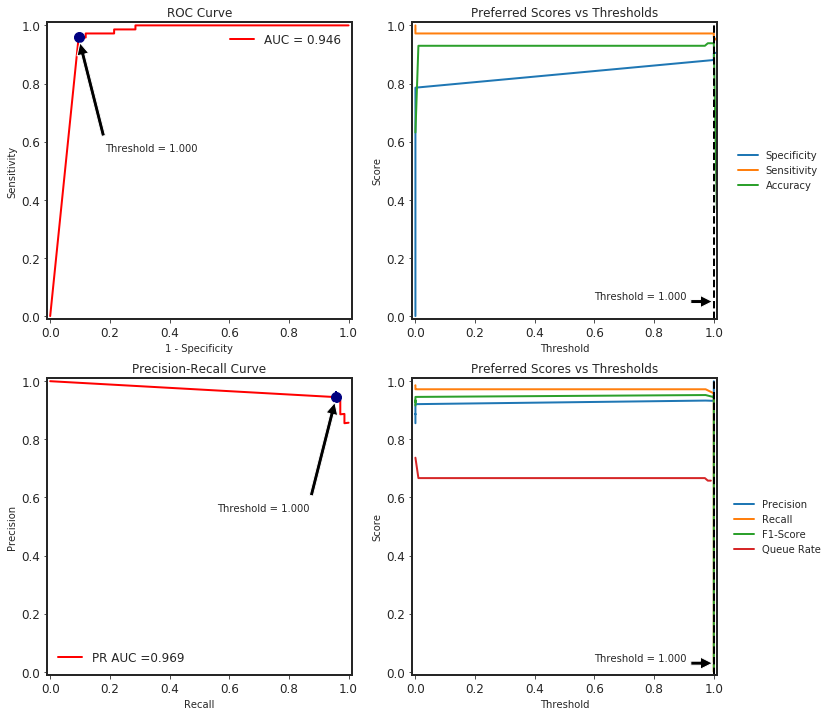
We can also calculate all the binary classification metrics using SlickML library.
# simply install slickml via pip
!pip install slickml
# loading BinaryClassificationMetrics
from slickml.metrics import BinaryClassificationMetrics
# initialize the metric object
clf_metrics = BinaryClassificationMetrics(y_test, y_pred_proba)
| Accuracy | Balanced Accuracy | ROC AUC | PR AUC | Precision | Recall | Average Precision | F-1 Score | F-2 Score | F-0.50 Score | Threat Score | TP | TN | FP | FN | |
|---|---|---|---|---|---|---|---|---|---|---|---|---|---|---|---|
| Threshold = 0.500 | Average = Binary | 0.930000 | 0.915000 | 0.946000 | 0.969000 | 0.921000 | 0.972000 | 0.943000 | 0.946000 | 0.962000 | 0.931000 | 0.897000 | 70 | 36 | 6 | 2 |
# plot roc, precision-recall with different thresholds calculations
clf_metrics.plot()