Imbalanced Classification

Imbalanced classification (or classification problems with low prevalence (low number of instances in one of the classes) can be challenging. In this post, I have discussed how we can model a problem with prevalence of 0.09% for positive class using gradient boosting and generalized linear model.
import numpy as np
import pandas as pd
import matplotlib.pyplot as plt
import matplotlib as mpl
from scipy import interp
from sklearn.preprocessing import scale
from sklearn.metrics import precision_score, recall_score, roc_auc_score, accuracy_score, roc_curve, auc, confusion_matrix
from sklearn.model_selection import cross_val_score, KFold, StratifiedKFold, train_test_split
from xgboost import XGBClassifier
import itertools
import glmnet
import xgboost as xgb
import shap
import seaborn as sns
sns.set_style("ticks")
mpl.rcParams['axes.linewidth'] = 3
mpl.rcParams['lines.linewidth'] =7
from IPython.core.display import display, HTML
display(HTML("<style>.container { width:95% !important; }</style>"))
import warnings
warnings.filterwarnings("ignore")
%matplotlib inline

# Unused Libraries here
# import keras
# from bayes_opt import BayesianOptimization
# from sklearn.model_selection import GridSearchCV, RandomizedSearchCV
# from fancyimpute import SoftImpute, IterativeImputer
Functions
#*-*-*-*-*-*-*-*-*-*-*-*-*-*-*-*-*-*-*-*-*-*-*-*-*-*-*-*-*-*-*-*-*-*-*-*-*-*-*-*-*-*-*-*-*-*-
# Function: _x_y_maker
def _x_y_maker(df, target, to_drop):
"""
A function to receive the dataframe and make the X, and Y matrices:
----------
parameters
input: dataframe df
string target (class label)
list[string] to_drop (list of columns need to be dropped)
output: dataframe Feature matrix (df_X)
Target vector (Y)
"""
Targets = df[target]
to_drop.append(target)
Features = df.drop(to_drop, axis = 1)
Scaled_Features = scale(Features.values)
df_X = pd.DataFrame(data = Scaled_Features, columns = Features.columns.tolist())
Y = Targets.values
return df_X, Y
#*-*-*-*-*-*-*-*-*-*-*-*-*-*-*-*-*-*-*-*-*-*-*-*-*-*-*-*-*-*-*-*-*-*-*-*-*-*-*-*-*-*-*-*-*-*-
# Function: _plot_roc_nfolds_xgboost
def _plot_roc_nfolds_xgboost(df_X, Y,
n_folds = 10,
n_estimators = 100,
learning_rate = 0.05,
max_depth = 3,
min_child_weight = 5.0,
gamma = 0.5,
reg_alpha = 0.0,
reg_lambda = 1.0,
subsample = 0.9,
objective = "binary:logistic",
scale_pos_weight = 1.0,
shuffle = True,
random_state = 1367
):
"""
a function to plot k-fold cv ROC using xgboost
input parameters:
df_X : features : pandas dataframe (numpy array will be built inside the function)
Y : targets
n_folds : number of cv folds (default = 10)
n_estimators = number of trees (default = 100)
learning_rate : step size of xgboost (default = 0.05)
max_depth : maximum tree depth for xgboost (default = 3)
min_child_weight : (default = 5.0)
gamma : (default = 0.5)
reg_alpha : lasso penalty (L1) (default = 0.0)
reg_lambda : ridge penalty (L2) (default = 1.0)
subsample : subsample fraction (default = 0.9)
objective : objective function for ML (default = "binary:logistic" for classification)
scale_pos_weight : (default = 1.0)
shuffle : shuffle flag for cv (default = True)
random_state : (default = 1367)
"""
# Defining the data
X = scale(df_X.values)
y = Y
n_samples, n_features = X.shape
# Run classifier with cross-validation and plot ROC curves
cv = StratifiedKFold(n_splits = n_folds , shuffle = shuffle , random_state = random_state)
classifier = XGBClassifier(learning_rate = learning_rate,
n_estimators = n_estimators,
max_depth = max_depth,
min_child_weight = min_child_weight,
gamma = gamma,
reg_alpha = reg_alpha,
reg_lambda = reg_lambda,
subsample = subsample,
objective = objective,
nthread = 4,
scale_pos_weight = 1.,
base_score = np.mean(y),
seed = random_state,
random_state = random_state)
tprs = []
aucs = []
mean_fpr = np.linspace(0, 1, 100)
plt.figure(figsize=(18 , 13))
i = 0
for train, test in cv.split(X, y):
probas_ = classifier.fit(X[train], y[train]).predict_proba(X[test])
# Compute ROC curve and area the curve
fpr, tpr, thresholds = roc_curve(y[test], probas_[:, 1])
tprs.append(interp(mean_fpr, fpr, tpr))
tprs[-1][0] = 0.0
roc_auc = auc(fpr, tpr)
aucs.append(roc_auc)
plt.plot(fpr, tpr, lw=3, alpha=0.5,
label="ROC Fold %d (AUC = %0.2f)" % (i+1, roc_auc))
i += 1
plt.plot([0, 1], [0, 1], linestyle="--", lw=3, color="k",
label="Luck", alpha=.8)
mean_tpr = np.mean(tprs, axis=0)
mean_tpr[-1] = 1.0
mean_auc = auc(mean_fpr, mean_tpr)
std_auc = np.std(aucs)
plt.plot(mean_fpr, mean_tpr, color="navy",
label=r"Mean ROC (AUC = %0.2f $\pm$ %0.2f)" % (mean_auc, std_auc),
lw=4)
std_tpr = np.std(tprs, axis=0)
tprs_upper = np.minimum(mean_tpr + std_tpr, 1)
tprs_lower = np.maximum(mean_tpr - std_tpr, 0)
plt.fill_between(mean_fpr, tprs_lower, tprs_upper, color="grey", alpha=.4,
label=r"$\pm$ 1 Standard Deviation")
plt.xlim([-0.05, 1.05])
plt.ylim([-0.05, 1.05])
plt.xlabel("False Positive Rate" , fontweight = "bold" , fontsize=30)
plt.ylabel("True Positive Rate",fontweight = "bold" , fontsize=30)
plt.tick_params(axis="both", which="major", labelsize=20)
plt.legend( prop={"size":20} , loc = 4)
# plt.savefig("./roc_xgboost.pdf" ,bbox_inches="tight")
plt.show()
#*-*-*-*-*-*-*-*-*-*-*-*-*-*-*-*-*-*-*-*-*-*-*-*-*-*-*-*-*-*-*-*-*-*-*-*-*-*-*-*-*-*-*-*-*-*-
# Function: _permute
def _permute(df, random_state):
"""
a funtion to permute the rows of features and add them
to the dataframe as noisy features to explore stability
input parameters:
df : pandas dataframe
random_state : random seed for noisy features
"""
normal_df = df.copy().reset_index(drop = True)
noisy_df = df.copy()
noisy_df.rename(columns = {col : "noisy_" + col for col in noisy_df.columns}, inplace = True)
np.random.seed(seed = random_state)
noisy_df = noisy_df.reindex(np.random.permutation(noisy_df.index))
merged_df = pd.concat([normal_df, noisy_df.reset_index(drop = True)] , axis = 1)
return merged_df
#*-*-*-*-*-*-*-*-*-*-*-*-*-*-*-*-*-*-*-*-*-*-*-*-*-*-*-*-*-*-*-*-*-*-*-*-*-*-*-*-*-*-*-*-*-*-
# Function: _my_feature_selector
def _my_feature_selector(X, Y, n_iter = 1,
num_boost_round = 1000,
nfold = 10,
stratified = True,
metrics = ("auc"),
early_stopping_rounds = 50,
seed = 1367,
shuffle = True,
show_stdv = False,
params = None,
importance_type = "total_gain",
callbacks = False,
verbose_eval = False):
"""
a function to run xgboost kfolds cv and train the model based on the best boosting round of each iteration.
for different number of iterations. at each iteration noisy features are added as well. at each iteration
internal and external cv calculated.
NOTE: it is recommended to use ad-hoc parameters to make sure the model is under-fitted for the sake of feature selection
input parameters:
X: features (pandas dataframe or numpy array)
Y: targets (1D array or list)
n_iter: total number of iterations (default = 1)
num_boost_rounds: max number of boosting rounds, (default = 1000)
stratified: stratificaiton of the targets (default = True)
metrics: classification/regression metrics (default = ("auc))
early_stopping_rounds: the criteria for stopping if the test metric is not improved (default = 20)
seed: random seed (default = 1367)
shuffle: shuffling the data (default = True)
show_stdv = showing standard deviation of cv results (default = False)
params = set of parameters for xgboost cv
(default_params = {
"eval_metric" : "auc",
"tree_method": "hist",
"objective" : "binary:logistic",
"learning_rate" : 0.05,
"max_depth": 2,
"min_child_weight": 1,
"gamma" : 0.0,
"reg_alpha" : 0.0,
"reg_lambda" : 1.0,
"subsample" : 0.9,
"max_delta_step": 1,
"silent" : 1,
"nthread" : 4,
"scale_pos_weight" : 1
}
)
importance_type = importance type of xgboost as string (default = "total_gain")
the other options will be "weight", "gain", "cover", and "total_cover"
callbacks = printing callbacks for xgboost cv
(defaults = False, if True: [xgb.callback.print_evaluation(show_stdv = show_stdv),
xgb.callback.early_stop(early_stopping_rounds)])
verbose_eval : a flag to show the result during train on train/test sets (default = False)
outputs:
outputs_dict: a dict contains the fitted models, internal and external cv results for train/test sets
df_selected: a dataframe contains feature names with their frequency of being selected at each run of folds
"""
# callback flag
if(callbacks == True):
callbacks = [xgb.callback.print_evaluation(show_stdv = show_stdv),
xgb.callback.early_stop(early_stopping_rounds)]
else:
callbacks = None
# params
default_params = {
"eval_metric" : "auc",
"tree_method": "hist",
"objective" : "binary:logistic",
"learning_rate" : 0.05,
"max_depth": 2,
"min_child_weight": 1,
"gamma" : 0.0,
"reg_alpha" : 0.0,
"reg_lambda" : 1.0,
"subsample" : 0.9,
"max_delta_step": 1,
"silent" : 1,
"nthread" : 4,
"scale_pos_weight" : 1,
"base_score" : np.mean(Y)
}
# updating the default parameters with the input
if params is not None:
for key, val in params.items():
default_params[key] = val
# total results list
int_cv_train = []
int_cv_test = []
ext_cv_train = []
ext_cv_test = []
bst_list = []
# main loop
for iteration in range(n_iter):
# results list at iteration
int_cv_train2 = []
int_cv_test2 = []
ext_cv_train2 = []
ext_cv_test2 = []
# update random state
random_state = seed * iteration
# adding noise to data
X_permuted = _permute(df = X, random_state = random_state)
cols = X_permuted.columns.tolist()
Xval = X_permuted.values
# building DMatrix for training/testing + kfolds cv
cv = StratifiedKFold(n_splits = nfold , shuffle = shuffle , random_state = random_state)
for train_index, test_index in cv.split(Xval, Y):
Xval_train = Xval[train_index]
Xval_test = Xval[test_index]
Y_train = Y[train_index]
Y_test = Y[test_index]
X_train = pd.DataFrame(data = Xval_train, columns = cols)
X_test = pd.DataFrame(data = Xval_test, columns = cols)
dtrain = xgb.DMatrix(data = X_train, label = Y_train)
dtest = xgb.DMatrix(data = X_test, label = Y_test)
# watchlist during final training
watchlist = [(dtrain,"train"), (dtest,"eval")]
# a dict to store training results
evals_result = {}
# xgb cv
cv_results = xgb.cv(params = default_params,
dtrain = dtrain,
num_boost_round = num_boost_round,
nfold = nfold,
stratified = stratified,
metrics = metrics,
early_stopping_rounds = early_stopping_rounds,
seed = random_state,
verbose_eval = verbose_eval,
shuffle = shuffle,
callbacks = callbacks)
int_cv_train.append(cv_results.iloc[-1][0])
int_cv_test.append(cv_results.iloc[-1][2])
int_cv_train2.append(cv_results.iloc[-1][0])
int_cv_test2.append(cv_results.iloc[-1][2])
# xgb train
bst = xgb.train(params = default_params,
dtrain = dtrain,
num_boost_round = len(cv_results) - 1,
evals = watchlist,
evals_result = evals_result,
verbose_eval = verbose_eval)
# appending outputs
bst_list.append(bst)
ext_cv_train.append(evals_result["train"]["auc"][-1])
ext_cv_test.append(evals_result["eval"]["auc"][-1])
ext_cv_train2.append(evals_result["train"]["auc"][-1])
ext_cv_test2.append(evals_result["eval"]["auc"][-1])
print(F"-*-*-*-*-*-*-*-*- Iteration {iteration + 1} -*-*-*-*-*-*-*-*")
print(F"-*-*- Internal-{nfold} Folds-CV-Train = {np.mean(int_cv_train2):.3} +/- {np.std(int_cv_train2):.3} -*-*- Internal-{nfold} Folds-CV-Test = {np.mean(int_cv_test2):.3} +/- {np.std(int_cv_test2):.3} -*-*")
print(F"-*-*- External-{nfold} Folds-CV-Train = {np.mean(ext_cv_train2):.3} +/- {np.std(ext_cv_train2):.3} -*-*- External-{nfold} Folds-CV-Test = {np.mean(ext_cv_test2):.3} +/- {np.std(ext_cv_test2):.3} -*-*")
# putting together the outputs in one dict
outputs = {}
outputs["bst"] = bst_list
outputs["int_cv_train"] = int_cv_train
outputs["int_cv_test"] = int_cv_test
outputs["ext_cv_train"] = ext_cv_train
outputs["ext_cv_test"] = ext_cv_test
pruned_features = []
for bst_ in outputs["bst"]:
features_gain = bst_.get_score(importance_type = importance_type)
for key, value in features_gain.items():
pruned_features.append(key)
unique_elements, counts_elements = np.unique(pruned_features, return_counts = True)
counts_elements = [float(i) for i in list(counts_elements)]
df_features = pd.DataFrame(data = {"columns" : list(unique_elements) , "count" : counts_elements})
df_features.sort_values(by = ["count"], ascending = False, inplace = True)
# plotting
plt.figure()
df_features.sort_values(by = ["count"]).plot.barh(x = "columns", y = "count", color = "pink" , figsize = (8,8))
plt.show()
plt.figure(figsize = (16,12))
plt.subplot(2,2,1)
plt.title(F"Internal {nfold} CV {metrics.upper()} - Train", fontsize = 20)
plt.hist(outputs["int_cv_train"], bins = 20, color = "lightgreen")
plt.subplot(2,2,2)
plt.title(F"Internal {nfold} CV {metrics.upper()} - Test", fontsize = 20)
plt.hist(outputs["int_cv_test"], bins = 20, color = "lightgreen")
plt.subplot(2,2,3)
plt.title(F"External {nfold} CV {metrics.upper()} - Train", fontsize = 20)
plt.hist(outputs["ext_cv_train"], bins = 20, color = "lightblue")
plt.subplot(2,2,4)
plt.title(F"External {nfold} CV {metrics.upper()} - Test", fontsize = 20)
plt.hist(outputs["ext_cv_test"], bins = 20, color = "lightblue")
plt.show()
return outputs, df_features
#*-*-*-*-*-*-*-*-*-*-*-*-*-*-*-*-*-*-*-*-*-*-*-*-*-*-*-*-*-*-*-*-*-*-*-*-*-*-*-*-*-*-*-*-*-*-
# Function: Confidence Interval calculator for 95% significance
def _ConfidenceInterval(score, n):
"""
confidence interval for 95% significance level
input: score such as accuracy, auc
the size of test set n
"""
CI_range = 1.96 * np.sqrt( (score * (1 - score)) / n)
CI_pos = score + CI_range
CI_neg = score - CI_range
if(CI_neg < 0):
CI_neg = 0
return CI_neg, CI_pos
#*-*-*-*-*-*-*-*-*-*-*-*-*-*-*-*-*-*-*-*-*-*-*-*-*-*-*-*-*-*-*-*-*-*-*-*-*-*-*-*-*-*-*-*-*-*-
# Function: _bst_shap
def _bst_shap(X, Y, num_boost_round = 1000,
nfold = 10,
stratified = True,
metrics = ("auc"),
early_stopping_rounds = 50,
seed = 1367,
shuffle = True,
show_stdv = False,
params = None,
callbacks = False):
"""
a function to run xgboost kfolds cv with the params and train the model based on best boosting rounds
input parameters:
X: features
Y: targets
num_boost_rounds: max number of boosting rounds, (default = 1000)
stratified: stratificaiton of the targets (default = True)
metrics: classification/regression metrics (default = ("auc))
early_stopping_rounds: the criteria for stopping if the test metric is not improved (default = 20)
seed: random seed (default = 1367)
shuffle: shuffling the data (default = True)
show_stdv = showing standard deviation of cv results (default = False)
params = set of parameters for xgboost cv ( default_params = {
"eval_metric" : "auc",
"tree_method": "hist",
"objective" : "binary:logistic",
"learning_rate" : 0.05,
"max_depth": 2,
"min_child_weight": 5,
"gamma" : 0.0,
"reg_alpha" : 0.0,
"reg_lambda" : 1.0,
"subsample" : 0.9,
"silent" : 1,
"nthread" : 4,
"scale_pos_weight" : 1
}
)
callbacks = printing callbacks for xgboost cv (defaults: [xgb.callback.print_evaluation(show_stdv = show_stdv),
xgb.callback.early_stop(early_stopping_rounds)])
outputs:
bst: the trained model based on optimum number of boosting rounds
cv_results: a dataframe contains the cv-results (train/test + std of train/test) for metric
"""
# callback flag
if(callbacks == True):
callbacks = [xgb.callback.print_evaluation(show_stdv = show_stdv),
xgb.callback.early_stop(early_stopping_rounds)]
else:
callbacks = None
# params
default_params = {
"eval_metric" : "auc",
"tree_method": "hist",
"objective" : "binary:logistic",
"learning_rate" : 0.05,
"max_depth": 2,
"min_child_weight": 1,
"gamma" : 0.0,
"reg_alpha" : 0.0,
"reg_lambda" : 1.0,
"subsample" : 0.9,
"max_delta_step": 1,
"silent" : 1,
"nthread" : 4
}
# updating the default parameters with the input
if params is not None:
for key, val in params.items():
default_params[key] = val
# building DMatrix for training
dtrain = xgb.DMatrix(data = X, label = Y)
print("-*-*-*-*-*-*-* CV Started *-*-*-*-*-*-*-")
cv_results = xgb.cv(params = default_params,
dtrain = dtrain,
num_boost_round = num_boost_round,
nfold = nfold,
stratified = stratified,
metrics = metrics,
early_stopping_rounds = early_stopping_rounds,
seed = seed,
shuffle = shuffle,
callbacks = callbacks)
print(F"*-*- Boosting Round = {len(cv_results) - 1} -*-*- Train = {cv_results.iloc[-1][0]:.3} -*-*- Test = {cv_results.iloc[-1][2]:.3} -*-*")
print("-*-*-*-*-*-*-* Train Started *-*-*-*-*-*-*-")
bst = xgb.train(params = default_params,
dtrain = dtrain,
num_boost_round = len(cv_results) - 1,
)
return bst, cv_results
#*-*-*-*-*-*-*-*-*-*-*-*-*-*-*-*-*-*-*-*-*-*-*-*-*-*-*-*-*-*-*-*-*-*-*-*-*-*-*-*-*-*-*-*-*-*-
# Function: _plot_xgboost_cv_score
def _plot_xgboost_cv_score(cv_results):
"""
a function to plot train/test cv score for
"""
import matplotlib as mpl
mpl.rcParams['axes.linewidth'] = 3
mpl.rcParams['lines.linewidth'] = 2
plt.figure(figsize=(10,8))
plt.errorbar(range(cv_results.shape[0]), cv_results["train-auc-mean"],
yerr=cv_results["train-auc-std"], fmt = "--", ecolor="lightgreen", c = "navy", label = "Train (9-Folds)")
plt.errorbar(range(cv_results.shape[0]), cv_results["test-auc-mean"],
yerr=cv_results["test-auc-std"], fmt = "--", ecolor="lightblue", c = "red", label = "Test (1-Fold)")
plt.xlabel("# of Boosting Rounds" , fontweight = "bold" , fontsize=30)
plt.ylabel("AUC",fontweight = "bold" , fontsize=30)
plt.tick_params(axis='both', which='major', labelsize=20)
plt.legend(loc = 4, prop={'size': 20})
plt.show()
#*-*-*-*-*-*-*-*-*-*-*-*-*-*-*-*-*-*-*-*-*-*-*-*-*-*-*-*-*-*-*-*-*-*-*-*-*-*-*-*-*-*-*-*-*-*-
# Function: _plot_importance
def _plot_importance(bst, importance_type = "total_gain", color = "pink", figsize = (10,10)):
"""
a function to plot feature importance in xgboost
"""
from xgboost import plot_importance
from pylab import rcParams
rcParams['figure.figsize'] = figsize
plot_importance(bst, importance_type = importance_type, color = color, xlabel = importance_type)
plt.show()
#*-*-*-*-*-*-*-*-*-*-*-*-*-*-*-*-*-*-*-*-*-*-*-*-*-*-*-*-*-*-*-*-*-*-*-*-*-*-*-*-*-*-*-*-*-*-
# Function: _plot_confusion_matrix
def _plot_confusion_matrix(cm, classes,
normalize=False,
title='Confusion matrix',
cmap=plt.cm.Greens):
"""
This function prints and plots the confusion matrix.
Normalization can be applied by setting `normalize=True`.
"""
if normalize:
cm = cm.astype('float') / cm.sum(axis=1)[:, np.newaxis]
print("Normalized confusion matrix")
else:
print('Confusion matrix, without normalization')
print(cm)
plt.imshow(cm, interpolation='nearest', cmap=cmap)
plt.title(title, fontsize = 20)
plt.colorbar()
tick_marks = np.arange(len(classes))
plt.xticks(tick_marks, classes)
plt.yticks(tick_marks, classes)
fmt = '.2f' if normalize else 'd'
thresh = cm.max() / 2.
for i, j in itertools.product(range(cm.shape[0]), range(cm.shape[1])):
plt.text(j, i, format(cm[i, j], fmt),
horizontalalignment="center",
color="white" if cm[i, j] > thresh else "black")
plt.ylabel('True label', fontsize = 20)
plt.xlabel('Predicted label', fontsize = 20)
plt.tick_params(axis='both', which='major', labelsize=20)
plt.tight_layout()
#*-*-*-*-*-*-*-*-*-*-*-*-*-*-*-*-*-*-*-*-*-*-*-*-*-*-*-*-*-*-*-*-*-*-*-*-*-*-*-*-*-*-*-*-*-*-
# Function: _clf_xgboost
def _clf_xgboost(df_X, Y, test_size, n_folds):
X = df_X.values
clf = XGBClassifier(learning_rate = 0.05,
n_estimators = 100,
max_depth = 3,
min_child_weight = 5.,
# max_delta_step= 1,
gamma = 0.5,
reg_alpha = 0.0,
reg_lambda = 1.0,
subsample = 0.9,
colsample_bytree = 0.9,
objective = "binary:logistic",
nthread = 4,
#scale_pos_weight = (len(Y) - sum(Y)) / sum(Y),
base_score = np.mean(Y),
seed = 1367,
random_state = 1367)
X_train, X_test, y_train, y_test = train_test_split(df_X, Y, test_size = test_size, shuffle = True, random_state = 1367, stratify = Y)
clf.fit(X_train, y_train, eval_metric="auc", early_stopping_rounds = 50, verbose = False, eval_set=[(X_test, y_test)])
accuracy_score = clf.score(X_test, y_test)
cv_roc_score = cross_val_score(clf, X, Y, cv = n_folds, scoring = "roc_auc")
y_pred_prob = clf.predict_proba(X_test)
roc_score = roc_auc_score(y_test, y_pred_prob[:,1])
fpr, tpr, thresholds = roc_curve(y_test, y_pred_prob[:,1])
optimal_idx = np.argmax(np.abs(tpr - fpr))
optimal_threshold = thresholds[optimal_idx]
return accuracy_score, roc_score, cv_roc_score, y_pred_prob, X_test, y_test, optimal_threshold
#*-*-*-*-*-*-*-*-*-*-*-*-*-*-*-*-*-*-*-*-*-*-*-*-*-*-*-*-*-*-*-*-*-*-*-*-*-*-*-*-*-*-*-*-*-*-
# Function: _xgboost_auc_hist
def _xgboost_auc_hist(df_X, Y, n_iterations = 100, alpha = 0.95):
"""
plot histogram of ROC AUC for N stratified classification for 95% significance level
"""
n_size = int(len(Y) * 0.30)
# Main Loop
scores = list()
for i in range(n_iterations):
# split the data into train/test sets
X_train, X_test, y_train, y_test = train_test_split(df_X, Y, test_size = n_size, shuffle = True, random_state = 1367 * i , stratify = Y)
# fit the xgboost classifier
clf = XGBClassifier(learning_rate = 0.05,
n_estimators = 100,
max_depth = 3,
min_child_weight = 5.,
# max_delta_step= 1,
gamma = 0.5,
reg_alpha = 0.0,
reg_lambda = 1.0,
subsample = 0.9,
colsample_bytree = 0.9,
objective = "binary:logistic",
nthread = 4,
#scale_pos_weight = (len(Y) - sum(Y)) / sum(Y),
base_score = np.mean(Y),
seed = 1367 * i ,
random_state = 1367 * i)
clf.fit(X_train, y_train, eval_metric = "auc", early_stopping_rounds = 50, verbose = False, eval_set = [(X_test, y_test)])
# evaluate model
predictions = clf.predict_proba(X_test)[:,1]
pred_auc = roc_auc_score(y_test, predictions)
scores.append(pred_auc)
# Ploting the scores
plt.figure(figsize=(10,5))
plt.hist(scores, color = "pink")
plt.xlabel("ROC AUC", fontsize = 30)
plt.tick_params(axis = "both", which = "major", labelsize = 15)
plt.show()
# confidence intervals
alpha = 0.95
p = ((1.0 - alpha)/2.0) * 100
lower = max(0.0, np.percentile(scores, p))
p = (alpha + ((1.0 - alpha)/2.0)) * 100
upper = min(1.0, np.percentile(scores, p))
print(F"{alpha*100}% Significance Level - ROC AUC Confidence Interval= [{lower:.3f} , {upper:.3f}]")
#*-*-*-*-*-*-*-*-*-*-*-*-*-*-*-*-*-*-*-*-*-*-*-*-*-*-*-*-*-*-*-*-*-*-*-*-*-*-*-*-*-*-*-*-*-*-
# Function: _glmnet
def _glmnet(X, Y, alpha = 0.1, n_splits = 10, scoring = "roc_auc"):
"""
a function for standard glmnet
input parameters: pandas dataframe X
class labels Y
alpha = 0.1
n_splits = 10
scoring = "roc_auc"
output: glmnet model
"""
model = glmnet.LogitNet(alpha = alpha,
n_lambda = 100,
n_splits = n_splits,
cut_point = 1.0,
scoring = scoring,
n_jobs = -1,
random_state = 1367)
model.fit(X, Y)
return model
#*-*-*-*-*-*-*-*-*-*-*-*-*-*-*-*-*-*-*-*-*-*-*-*-*-*-*-*-*-*-*-*-*-*-*-*-*-*-*-*-*-*-*-*-*-*-
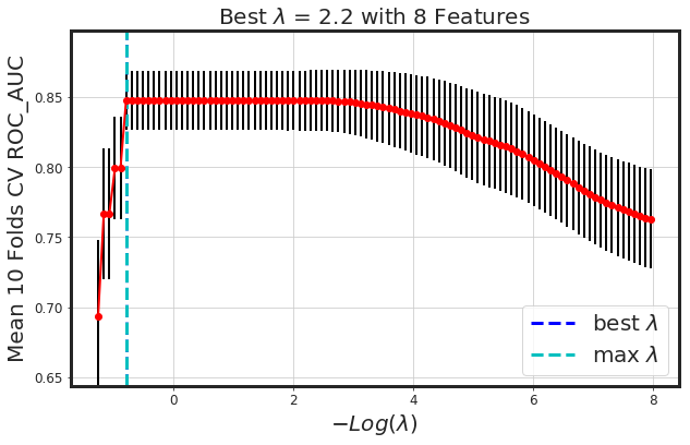
# Function: _plot_glmnet_cv_score
def _plot_glmnet_cv_score(model):
"""
a function to plot cv scores vs lambda
parameters:
model : a fitted glmnet object
"""
mpl.rcParams['axes.linewidth'] = 3
mpl.rcParams['lines.linewidth'] =2
plt.figure(figsize=(10,6))
plt.errorbar(-np.log(model.lambda_path_), model.cv_mean_score_, yerr=model.cv_standard_error_ , c = "r", ecolor="k", marker = "o" )
plt.vlines(-np.log(model.lambda_best_), ymin = min(model.cv_mean_score_) - 0.05 , ymax = max(model.cv_mean_score_) + 0.05, lw = 3, linestyles = "--", colors = "b" ,label = "best $\lambda$")
plt.vlines(-np.log(model.lambda_max_), ymin = min(model.cv_mean_score_) - 0.05 , ymax = max(model.cv_mean_score_) + 0.05, lw = 3, linestyles = "--", colors = "c" ,label = "max $\lambda$")
plt.tick_params(axis='both', which='major', labelsize = 12)
plt.grid(True)
plt.ylim([min(model.cv_mean_score_) - 0.05, max(model.cv_mean_score_) + 0.05])
plt.legend(loc = 4, prop={'size': 20})
plt.xlabel("$-Log(\lambda)$" , fontsize = 20)
plt.ylabel(F"Mean {model.n_splits} Folds CV {(model.scoring).upper()}", fontsize = 20)
plt.title(F"Best $\lambda$ = {model.lambda_best_[0]:.2} with {len(np.nonzero( model.coef_)[1])} Features" , fontsize = 20)
plt.show()
#*-*-*-*-*-*-*-*-*-*-*-*-*-*-*-*-*-*-*-*-*-*-*-*-*-*-*-*-*-*-*-*-*-*-*-*-*-*-*-*-*-*-*-*-*-*-
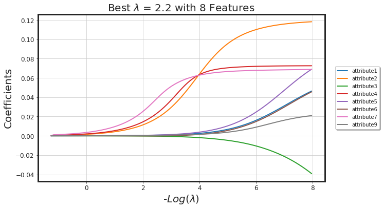
# Function: _plot_glmnet_coeff_path
def _plot_glmnet_coeff_path(model, df):
"""
a function to plot coefficients vs lambda
parameters:
model : a fitted glmnet object
df: in case that the input is the pandas dataframe,
the column names of the coeff. will appear as a legend
"""
mpl.rcParams['axes.linewidth'] = 3
mpl.rcParams['lines.linewidth'] =2
plt.figure(figsize=(10,6))
if not df.empty:
for i in list(np.nonzero(np.reshape(model.coef_, (1,-1)))[1]):
plt.plot(-np.log(model.lambda_path_) ,(model.coef_path_.reshape(-1,model.coef_path_.shape[-1]))[i,:], label = df.columns.values.tolist()[i]);
plt.legend(loc= "right", bbox_to_anchor=(1.2 , .5), ncol=1, fancybox=True, shadow=True)
else:
for i in list(np.nonzero(np.reshape(model.coef_, (1,-1)))[1]):
plt.plot(-np.log(model.lambda_path_) ,(model.coef_path_.reshape(-1, model.coef_path_.shape[-1]))[i,:]);
plt.tick_params(axis='both', which='major', labelsize = 12)
plt.ylabel("Coefficients", fontsize = 20)
plt.xlabel("-$Log(\lambda)$", fontsize = 20)
plt.title(F"Best $\lambda$ = {model.lambda_best_[0]:.2} with {len(np.nonzero(model.coef_)[1])} Features" , fontsize = 20)
plt.grid(True)
plt.show()
#*-*-*-*-*-*-*-*-*-*-*-*-*-*-*-*-*-*-*-*-*-*-*-*-*-*-*-*-*-*-*-*-*-*-*-*-*-*-*-*-*-*-*-*-*-*-
# Function: _df_glmnet_coeff_path
def _df_glmnet_coeff_path(model, df):
"""
a function to build a dataframe for nonzero coeff.
parameters:
model : a fitted glmnet object
df: in case that the input is the pandas dataframe,
the column names of the coeff. will appear as a legend
"""
idx = list(np.nonzero(np.reshape(model.coef_, (1,-1)))[1])
dct = dict( zip([df.columns.tolist()[i] for i in idx], [model.coef_[0][i] for i in idx]))
return pd.DataFrame(data = dct.items() , columns = ["Features", "Coeffs"]).sort_values(by = "Coeffs", ascending = False).reset_index(drop = True)
#*-*-*-*-*-*-*-*-*-*-*-*-*-*-*-*-*-*-*-*-*-*-*-*-*-*-*-*-*-*-*-*-*-*-*-*-*-*-*-*-*-*-*-*-*-*-
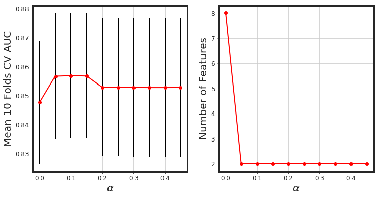
# Function: _glmnet_best_score_alpha
def _glmnet_best_score_alpha(X, Y):
"""
a function to run glmnet for different alpha
"""
def logitnet_nonzero_coef(g):
idx = np.where(g.coef_[0] != 0)[0]
return pd.DataFrame({"idx": idx, "coef": g.coef_[0][idx]})
alpha_list = np.arange(0.0, 0.5, 0.05)
mean_auc = []
std_auc = []
n_features = []
for alpha in alpha_list:
model = _glmnet(X, Y, alpha = alpha)
mean_auc.append(model.cv_mean_score_[model.lambda_best_inx_])
std_auc.append(model.cv_standard_error_[model.lambda_best_inx_])
fe = logitnet_nonzero_coef(model)
n_features.append(fe.shape[0])
mpl.rcParams['axes.linewidth'] = 3
mpl.rcParams['lines.linewidth'] =2
plt.figure(figsize=(12,6))
plt.subplot(1,2,1)
plt.errorbar(alpha_list, mean_auc, yerr = std_auc, c = "r", ecolor="k", marker = "o" )
plt.tick_params(axis='both', which='major', labelsize = 12)
plt.xlabel(r"$\alpha$" , fontsize = 20)
plt.ylabel("Mean 10 Folds CV AUC", fontsize = 20)
plt.grid(True)
plt.subplot(1,2,2)
plt.plot(alpha_list, n_features, c = "r", marker = "o" )
plt.tick_params(axis='both', which='major', labelsize = 12)
plt.xlabel(r"$\alpha$" , fontsize = 20)
plt.ylabel("Number of Features", fontsize = 20)
plt.grid(True)
plt.show()
First, I loaded the data into a pandas dataframe to get some idea.
# readin the data into a dataframe
dateparser = lambda x: pd.datetime.strptime(x, "%Y-%m-%d")
df_raw = pd.read_csv("./device_failure.csv",
                     parse_dates = ["date"],
                     date_parser = dateparser,
                     encoding = "cp1252")
print("Shape: {}".format(df_raw.shape))
print("Prevalence = {:.3f}%".format(df_raw["failure"].sum()/df_raw.shape[0] * 100))
Shape: (124494, 12)
Prevalence = 0.085%
df_raw.head()
| date | device | failure | attribute1 | attribute2 | attribute3 | attribute4 | attribute5 | attribute6 | attribute7 | attribute8 | attribute9 | |
|---|---|---|---|---|---|---|---|---|---|---|---|---|
| 0 | 2015-01-01 | S1F01085 | 0 | 215630672 | 56 | 0 | 52 | 6 | 407438 | 0 | 0 | 7 |
| 1 | 2015-01-01 | S1F0166B | 0 | 61370680 | 0 | 3 | 0 | 6 | 403174 | 0 | 0 | 0 |
| 2 | 2015-01-01 | S1F01E6Y | 0 | 173295968 | 0 | 0 | 0 | 12 | 237394 | 0 | 0 | 0 |
| 3 | 2015-01-01 | S1F01JE0 | 0 | 79694024 | 0 | 0 | 0 | 6 | 410186 | 0 | 0 | 0 |
| 4 | 2015-01-01 | S1F01R2B | 0 | 135970480 | 0 | 0 | 0 | 15 | 313173 | 0 | 0 | 3 |
Printing out the statistical description of the data. It would help us to have idea about the variation of the each column in the data.
df_raw.describe()
| failure | attribute1 | attribute2 | attribute3 | attribute4 | attribute5 | attribute6 | attribute7 | attribute8 | attribute9 | |
|---|---|---|---|---|---|---|---|---|---|---|
| count | 124494.000000 | 1.244940e+05 | 124494.000000 | 124494.000000 | 124494.000000 | 124494.000000 | 124494.000000 | 124494.000000 | 124494.000000 | 124494.000000 |
| mean | 0.000851 | 1.223881e+08 | 159.484762 | 9.940455 | 1.741120 | 14.222669 | 260172.657726 | 0.292528 | 0.292528 | 12.451524 |
| std | 0.029167 | 7.045933e+07 | 2179.657730 | 185.747321 | 22.908507 | 15.943028 | 99151.078547 | 7.436924 | 7.436924 | 191.425623 |
| min | 0.000000 | 0.000000e+00 | 0.000000 | 0.000000 | 0.000000 | 1.000000 | 8.000000 | 0.000000 | 0.000000 | 0.000000 |
| 25% | 0.000000 | 6.128476e+07 | 0.000000 | 0.000000 | 0.000000 | 8.000000 | 221452.000000 | 0.000000 | 0.000000 | 0.000000 |
| 50% | 0.000000 | 1.227974e+08 | 0.000000 | 0.000000 | 0.000000 | 10.000000 | 249799.500000 | 0.000000 | 0.000000 | 0.000000 |
| 75% | 0.000000 | 1.833096e+08 | 0.000000 | 0.000000 | 0.000000 | 12.000000 | 310266.000000 | 0.000000 | 0.000000 | 0.000000 |
| max | 1.000000 | 2.441405e+08 | 64968.000000 | 24929.000000 | 1666.000000 | 98.000000 | 689161.000000 | 832.000000 | 832.000000 | 18701.000000 |
Printing out the number of Null values in each column. These numbers should be imputed before feeding into the classifier.
df_raw.isnull().sum()
date          0
device        0
failure       0
attribute1    0
attribute2    0
attribute3    0
attribute4    0
attribute5    0
attribute6    0
attribute7    0
attribute8    0
attribute9    0
dtype: int64
Checking the data types of the columns to make sure all the columns have continuous values as it is mentioned in the meta data, except date and device
df_raw.dtypes
date          datetime64[ns]
device                object
failure                int64
attribute1             int64
attribute2             int64
attribute3             int64
attribute4             int64
attribute5             int64
attribute6             int64
attribute7             int64
attribute8             int64
attribute9             int64
dtype: object
Checking the pair-wise correlation between features
methods = {‘pearson’, ‘kendall’, ‘spearman’}
df_raw.corr(method = "kendall")
| failure | attribute1 | attribute2 | attribute3 | attribute4 | attribute5 | attribute6 | attribute7 | attribute8 | attribute9 | |
|---|---|---|---|---|---|---|---|---|---|---|
| failure | 1.000000 | 0.001611 | 0.053361 | 0.003208 | 0.057295 | 0.003475 | 0.002337 | 0.096926 | 0.096926 | 0.004633 |
| attribute1 | 0.001611 | 1.000000 | -0.001004 | 0.001960 | 0.001289 | -0.003713 | -0.001779 | -0.002030 | -0.002030 | -0.002662 |
| attribute2 | 0.053361 | -0.001004 | 1.000000 | -0.018322 | 0.219415 | -0.022125 | -0.062126 | 0.107491 | 0.107491 | -0.027759 |
| attribute3 | 0.003208 | 0.001960 | -0.018322 | 1.000000 | 0.117459 | 0.089091 | 0.056736 | -0.009622 | -0.009622 | 0.369092 |
| attribute4 | 0.057295 | 0.001289 | 0.219415 | 0.117459 | 1.000000 | -0.017980 | 0.009706 | 0.160216 | 0.160216 | 0.046189 |
| attribute5 | 0.003475 | -0.003713 | -0.022125 | 0.089091 | -0.017980 | 1.000000 | 0.057295 | -0.016603 | -0.016603 | 0.026998 |
| attribute6 | 0.002337 | -0.001779 | -0.062126 | 0.056736 | 0.009706 | 0.057295 | 1.000000 | -0.013186 | -0.013186 | 0.069585 |
| attribute7 | 0.096926 | -0.002030 | 0.107491 | -0.009622 | 0.160216 | -0.016603 | -0.013186 | 1.000000 | 1.000000 | -0.017097 |
| attribute8 | 0.096926 | -0.002030 | 0.107491 | -0.009622 | 0.160216 | -0.016603 | -0.013186 | 1.000000 | 1.000000 | -0.017097 |
| attribute9 | 0.004633 | -0.002662 | -0.027759 | 0.369092 | 0.046189 | 0.026998 | 0.069585 | -0.017097 | -0.017097 | 1.000000 |
# Number of unique devices: this can be used as feauture based on the demand
df_raw["device"].nunique()
1169
Preprocessing: attribute7 and attribute8 are totally correlated (the same feature). For now, I am gonna drop date and device as well. Device has 1169 unique values that can be used as features.
df = df_raw.copy()
target = "failure"
to_drop = ["date", "device", "attribute8"]
df_X, Y = _x_y_maker(df, target, to_drop)
Printing the first 5 rows of the sclaed features.
df_X.head()
| attribute1 | attribute2 | attribute3 | attribute4 | attribute5 | attribute6 | attribute7 | attribute9 | |
|---|---|---|---|---|---|---|---|---|
| 0 | 1.323358 | -0.047478 | -0.053516 | 2.193905 | -0.515755 | 1.485268 | -0.039335 | -0.028479 |
| 1 | -0.865998 | -0.073170 | -0.037365 | -0.076004 | -0.515755 | 1.442263 | -0.039335 | -0.065047 |
| 2 | 0.722517 | -0.073170 | -0.053516 | -0.076004 | -0.139414 | -0.229738 | -0.039335 | -0.065047 |
| 3 | -0.605942 | -0.073170 | -0.053516 | -0.076004 | -0.515755 | 1.512983 | -0.039335 | -0.065047 |
| 4 | 0.192770 | -0.073170 | -0.053516 | -0.076004 | 0.048757 | 0.534543 | -0.039335 | -0.049375 |
Checking the correlation again.
df_X.corr()
| attribute1 | attribute2 | attribute3 | attribute4 | attribute5 | attribute6 | attribute7 | attribute9 | |
|---|---|---|---|---|---|---|---|---|
| attribute1 | 1.000000 | -0.004250 | 0.003701 | 0.001836 | -0.003376 | -0.001522 | 0.000151 | 0.001121 |
| attribute2 | -0.004250 | 1.000000 | -0.002617 | 0.146593 | -0.013999 | -0.026350 | 0.141367 | -0.002736 |
| attribute3 | 0.003701 | -0.002617 | 1.000000 | 0.097452 | -0.006696 | 0.009027 | -0.001884 | 0.532366 |
| attribute4 | 0.001836 | 0.146593 | 0.097452 | 1.000000 | -0.009773 | 0.024870 | 0.045631 | 0.036069 |
| attribute5 | -0.003376 | -0.013999 | -0.006696 | -0.009773 | 1.000000 | -0.017049 | -0.009384 | 0.005949 |
| attribute6 | -0.001522 | -0.026350 | 0.009027 | 0.024870 | -0.017049 | 1.000000 | -0.012207 | 0.021152 |
| attribute7 | 0.000151 | 0.141367 | -0.001884 | 0.045631 | -0.009384 | -0.012207 | 1.000000 | 0.006861 |
| attribute9 | 0.001121 | -0.002736 | 0.532366 | 0.036069 | 0.005949 | 0.021152 | 0.006861 | 1.000000 |
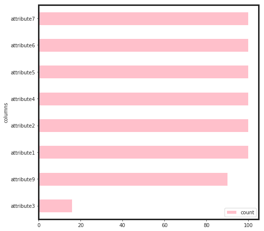
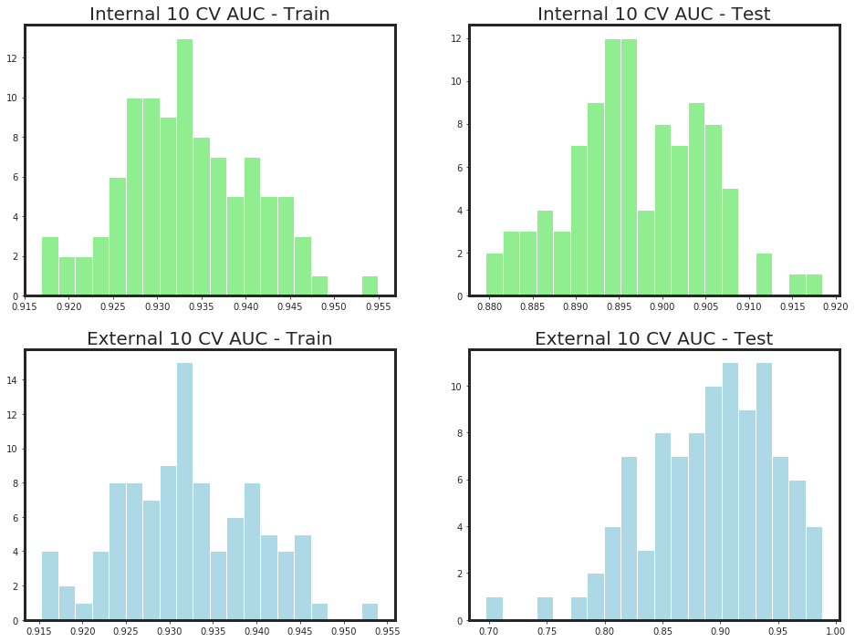
Running my feature selector along with noise with 10-folds CV for multiple iterations to make sure about the selected features. This would help to have a simpler model with the same performance
# choosing params to under-fit the model for feature selection + noisy features. This would help to have simpler model
params = {
          "learning_rate" : 0.05,
          "max_depth": 2,
          "min_child_weight": 5,
          "gamma" : 0.5

         }
o_, d_ = _my_feature_selector(df_X, Y, n_iter = 10,
                                       params = params,
                                       seed = 1367,
                                       callbacks = False)
-*-*-*-*-*-*-*-*- Iteration 1 -*-*-*-*-*-*-*-*
-*-*- Internal-10 Folds-CV-Train = 0.935 +/- 0.00485 -*-*- Internal-10 Folds-CV-Test = 0.897 +/- 0.00849 -*-*
-*-*- External-10 Folds-CV-Train = 0.933 +/- 0.005 -*-*- External-10 Folds-CV-Test = 0.898 +/- 0.0435 -*-*
-*-*-*-*-*-*-*-*- Iteration 2 -*-*-*-*-*-*-*-*
-*-*- Internal-10 Folds-CV-Train = 0.932 +/- 0.00891 -*-*- Internal-10 Folds-CV-Test = 0.896 +/- 0.00948 -*-*
-*-*- External-10 Folds-CV-Train = 0.931 +/- 0.00924 -*-*- External-10 Folds-CV-Test = 0.892 +/- 0.0413 -*-*
-*-*-*-*-*-*-*-*- Iteration 3 -*-*-*-*-*-*-*-*
-*-*- Internal-10 Folds-CV-Train = 0.934 +/- 0.0065 -*-*- Internal-10 Folds-CV-Test = 0.896 +/- 0.00591 -*-*
-*-*- External-10 Folds-CV-Train = 0.933 +/- 0.00634 -*-*- External-10 Folds-CV-Test = 0.892 +/- 0.0571 -*-*
-*-*-*-*-*-*-*-*- Iteration 4 -*-*-*-*-*-*-*-*
-*-*- Internal-10 Folds-CV-Train = 0.935 +/- 0.00669 -*-*- Internal-10 Folds-CV-Test = 0.897 +/- 0.00905 -*-*
-*-*- External-10 Folds-CV-Train = 0.933 +/- 0.00776 -*-*- External-10 Folds-CV-Test = 0.894 +/- 0.0548 -*-*
-*-*-*-*-*-*-*-*- Iteration 5 -*-*-*-*-*-*-*-*
-*-*- Internal-10 Folds-CV-Train = 0.934 +/- 0.00684 -*-*- Internal-10 Folds-CV-Test = 0.897 +/- 0.00607 -*-*
-*-*- External-10 Folds-CV-Train = 0.932 +/- 0.00653 -*-*- External-10 Folds-CV-Test = 0.894 +/- 0.052 -*-*
-*-*-*-*-*-*-*-*- Iteration 6 -*-*-*-*-*-*-*-*
-*-*- Internal-10 Folds-CV-Train = 0.932 +/- 0.0068 -*-*- Internal-10 Folds-CV-Test = 0.898 +/- 0.0082 -*-*
-*-*- External-10 Folds-CV-Train = 0.931 +/- 0.00678 -*-*- External-10 Folds-CV-Test = 0.892 +/- 0.0493 -*-*
-*-*-*-*-*-*-*-*- Iteration 7 -*-*-*-*-*-*-*-*
-*-*- Internal-10 Folds-CV-Train = 0.931 +/- 0.0071 -*-*- Internal-10 Folds-CV-Test = 0.896 +/- 0.00643 -*-*
-*-*- External-10 Folds-CV-Train = 0.93 +/- 0.00858 -*-*- External-10 Folds-CV-Test = 0.892 +/- 0.0339 -*-*
-*-*-*-*-*-*-*-*- Iteration 8 -*-*-*-*-*-*-*-*
-*-*- Internal-10 Folds-CV-Train = 0.933 +/- 0.00951 -*-*- Internal-10 Folds-CV-Test = 0.898 +/- 0.00782 -*-*
-*-*- External-10 Folds-CV-Train = 0.932 +/- 0.00995 -*-*- External-10 Folds-CV-Test = 0.892 +/- 0.0766 -*-*
-*-*-*-*-*-*-*-*- Iteration 9 -*-*-*-*-*-*-*-*
-*-*- Internal-10 Folds-CV-Train = 0.929 +/- 0.00658 -*-*- Internal-10 Folds-CV-Test = 0.895 +/- 0.00973 -*-*
-*-*- External-10 Folds-CV-Train = 0.928 +/- 0.00671 -*-*- External-10 Folds-CV-Test = 0.896 +/- 0.0523 -*-*
-*-*-*-*-*-*-*-*- Iteration 10 -*-*-*-*-*-*-*-*
-*-*- Internal-10 Folds-CV-Train = 0.935 +/- 0.00538 -*-*- Internal-10 Folds-CV-Test = 0.898 +/- 0.00774 -*-*
-*-*- External-10 Folds-CV-Train = 0.933 +/- 0.0058 -*-*- External-10 Folds-CV-Test = 0.883 +/- 0.0507 -*-*


<Figure size 432x288 with 0 Axes>
params = {
          "learning_rate" : 0.05,
          "max_depth": 2,
          "min_child_weight": 5.,
          "gamma" : 0.5
         }
bst, cvr = _bst_shap(df_X, Y, params = params, callbacks = True)
-*-*-*-*-*-*-* CV Started *-*-*-*-*-*-*-
[22:09:38] Tree method is selected to be 'hist', which uses a single updater grow_fast_histmaker.
[22:09:38] Tree method is selected to be 'hist', which uses a single updater grow_fast_histmaker.
[22:09:38] Tree method is selected to be 'hist', which uses a single updater grow_fast_histmaker.
[22:09:39] Tree method is selected to be 'hist', which uses a single updater grow_fast_histmaker.
[22:09:39] Tree method is selected to be 'hist', which uses a single updater grow_fast_histmaker.
[22:09:39] Tree method is selected to be 'hist', which uses a single updater grow_fast_histmaker.
[22:09:39] Tree method is selected to be 'hist', which uses a single updater grow_fast_histmaker.
[22:09:39] Tree method is selected to be 'hist', which uses a single updater grow_fast_histmaker.
[22:09:39] Tree method is selected to be 'hist', which uses a single updater grow_fast_histmaker.
[22:09:39] Tree method is selected to be 'hist', which uses a single updater grow_fast_histmaker.
[0] train-auc:0.5 test-auc:0.5
Multiple eval metrics have been passed: 'test-auc' will be used for early stopping.
Will train until test-auc hasn't improved in 50 rounds.
[1] train-auc:0.5 test-auc:0.5
[2] train-auc:0.5 test-auc:0.5
[3] train-auc:0.5 test-auc:0.5
[4] train-auc:0.5 test-auc:0.5
[5] train-auc:0.5 test-auc:0.5
[6] train-auc:0.5 test-auc:0.5
[7] train-auc:0.5 test-auc:0.5
[8] train-auc:0.5 test-auc:0.5
[9] train-auc:0.5 test-auc:0.5
[10] train-auc:0.5 test-auc:0.5
[11] train-auc:0.5 test-auc:0.5
[12] train-auc:0.5 test-auc:0.5
[13] train-auc:0.5 test-auc:0.5
[14] train-auc:0.5 test-auc:0.5
[15] train-auc:0.5 test-auc:0.5
[16] train-auc:0.5 test-auc:0.5
[17] train-auc:0.5 test-auc:0.5
[18] train-auc:0.502591 test-auc:0.499988
[19] train-auc:0.507799 test-auc:0.499972
[20] train-auc:0.515655 test-auc:0.499924
[21] train-auc:0.515655 test-auc:0.499924
[22] train-auc:0.521354 test-auc:0.504899
[23] train-auc:0.527633 test-auc:0.509397
[24] train-auc:0.544239 test-auc:0.51922
[25] train-auc:0.547894 test-auc:0.519192
[26] train-auc:0.562889 test-auc:0.528576
[27] train-auc:0.562888 test-auc:0.528573
[28] train-auc:0.575345 test-auc:0.551115
[29] train-auc:0.589815 test-auc:0.570037
[30] train-auc:0.589813 test-auc:0.570032
[31] train-auc:0.589815 test-auc:0.570038
[32] train-auc:0.594991 test-auc:0.579028
[33] train-auc:0.603815 test-auc:0.588018
[34] train-auc:0.607991 test-auc:0.587983
[35] train-auc:0.607994 test-auc:0.587977
[36] train-auc:0.609034 test-auc:0.587952
[37] train-auc:0.611603 test-auc:0.58792
[38] train-auc:0.611606 test-auc:0.58792
[39] train-auc:0.621348 test-auc:0.592728
[40] train-auc:0.630541 test-auc:0.59751
[41] train-auc:0.641352 test-auc:0.610898
[42] train-auc:0.645456 test-auc:0.619846
[43] train-auc:0.649023 test-auc:0.624774
[44] train-auc:0.649023 test-auc:0.629293
[45] train-auc:0.652603 test-auc:0.638277
[46] train-auc:0.656164 test-auc:0.638207
[47] train-auc:0.656163 test-auc:0.638208
[48] train-auc:0.660153 test-auc:0.638036
[49] train-auc:0.660154 test-auc:0.638033
[50] train-auc:0.668212 test-auc:0.637722
[51] train-auc:0.683198 test-auc:0.651949
[52] train-auc:0.68676 test-auc:0.65183
[53] train-auc:0.702173 test-auc:0.664918
[54] train-auc:0.705216 test-auc:0.673904
[55] train-auc:0.716932 test-auc:0.688166
[56] train-auc:0.746947 test-auc:0.705966
[57] train-auc:0.766238 test-auc:0.732417
[58] train-auc:0.76625 test-auc:0.732301
[59] train-auc:0.781952 test-auc:0.749171
[60] train-auc:0.785332 test-auc:0.753368
[61] train-auc:0.788794 test-auc:0.753104
[62] train-auc:0.788767 test-auc:0.753255
[63] train-auc:0.789759 test-auc:0.757569
[64] train-auc:0.789792 test-auc:0.757407
[65] train-auc:0.791717 test-auc:0.762459
[66] train-auc:0.791741 test-auc:0.762543
[67] train-auc:0.794139 test-auc:0.771179
[68] train-auc:0.79414 test-auc:0.771128
[69] train-auc:0.798393 test-auc:0.78537
[70] train-auc:0.799311 test-auc:0.790212
[71] train-auc:0.799362 test-auc:0.790179
[72] train-auc:0.799436 test-auc:0.790156
[73] train-auc:0.804061 test-auc:0.789724
[74] train-auc:0.809716 test-auc:0.793472
[75] train-auc:0.81023 test-auc:0.793571
[76] train-auc:0.810291 test-auc:0.793676
[77] train-auc:0.810273 test-auc:0.794129
[78] train-auc:0.815368 test-auc:0.793779
[79] train-auc:0.818557 test-auc:0.798271
[80] train-auc:0.818553 test-auc:0.798253
[81] train-auc:0.818556 test-auc:0.798244
[82] train-auc:0.819048 test-auc:0.798204
[83] train-auc:0.819046 test-auc:0.798256
[84] train-auc:0.819084 test-auc:0.798343
[85] train-auc:0.819094 test-auc:0.798331
[86] train-auc:0.826427 test-auc:0.810713
[87] train-auc:0.827297 test-auc:0.815134
[88] train-auc:0.827317 test-auc:0.820203
[89] train-auc:0.82735 test-auc:0.820224
[90] train-auc:0.835594 test-auc:0.836472
[91] train-auc:0.839335 test-auc:0.83642
[92] train-auc:0.839334 test-auc:0.836343
[93] train-auc:0.844798 test-auc:0.840614
[94] train-auc:0.845237 test-auc:0.840554
[95] train-auc:0.845206 test-auc:0.840589
[96] train-auc:0.845202 test-auc:0.840541
[97] train-auc:0.845634 test-auc:0.840411
[98] train-auc:0.846109 test-auc:0.840341
[99] train-auc:0.8461 test-auc:0.840213
[100] train-auc:0.846579 test-auc:0.840174
[101] train-auc:0.847455 test-auc:0.840033
[102] train-auc:0.848847 test-auc:0.839937
[103] train-auc:0.848889 test-auc:0.839934
[104] train-auc:0.851638 test-auc:0.839058
[105] train-auc:0.851658 test-auc:0.839094
[106] train-auc:0.851696 test-auc:0.839025
[107] train-auc:0.851761 test-auc:0.839107
[108] train-auc:0.855548 test-auc:0.838203
[109] train-auc:0.855952 test-auc:0.838216
[110] train-auc:0.859843 test-auc:0.837271
[111] train-auc:0.859896 test-auc:0.837218
[112] train-auc:0.862772 test-auc:0.844197
[113] train-auc:0.866681 test-auc:0.847177
[114] train-auc:0.866765 test-auc:0.847206
[115] train-auc:0.867214 test-auc:0.847115
[116] train-auc:0.868626 test-auc:0.855585
[117] train-auc:0.869564 test-auc:0.859661
[118] train-auc:0.869588 test-auc:0.859604
[119] train-auc:0.870008 test-auc:0.859496
[120] train-auc:0.870083 test-auc:0.859439
[121] train-auc:0.870515 test-auc:0.859276
[122] train-auc:0.871057 test-auc:0.859007
[123] train-auc:0.871131 test-auc:0.859277
[124] train-auc:0.871211 test-auc:0.859541
[125] train-auc:0.871218 test-auc:0.859699
[126] train-auc:0.871588 test-auc:0.863687
[127] train-auc:0.871767 test-auc:0.863805
[128] train-auc:0.87185 test-auc:0.864008
[129] train-auc:0.871903 test-auc:0.863906
[130] train-auc:0.871946 test-auc:0.863755
[131] train-auc:0.871992 test-auc:0.863533
[132] train-auc:0.87198 test-auc:0.863675
[133] train-auc:0.872139 test-auc:0.863535
[134] train-auc:0.872082 test-auc:0.86365
[135] train-auc:0.872188 test-auc:0.863516
[136] train-auc:0.872232 test-auc:0.86354
[137] train-auc:0.872228 test-auc:0.863652
[138] train-auc:0.872266 test-auc:0.863696
[139] train-auc:0.872255 test-auc:0.863683
[140] train-auc:0.872303 test-auc:0.863636
[141] train-auc:0.872336 test-auc:0.863547
[142] train-auc:0.872402 test-auc:0.863523
[143] train-auc:0.872441 test-auc:0.863512
[144] train-auc:0.876281 test-auc:0.865899
[145] train-auc:0.876307 test-auc:0.865908
[146] train-auc:0.876324 test-auc:0.86593
[147] train-auc:0.876275 test-auc:0.870426
[148] train-auc:0.876311 test-auc:0.8704
[149] train-auc:0.876318 test-auc:0.870282
[150] train-auc:0.876344 test-auc:0.870302
[151] train-auc:0.876323 test-auc:0.87028
[152] train-auc:0.876347 test-auc:0.870184
[153] train-auc:0.876402 test-auc:0.87025
[154] train-auc:0.876392 test-auc:0.870155
[155] train-auc:0.876437 test-auc:0.870074
[156] train-auc:0.876463 test-auc:0.870078
[157] train-auc:0.884578 test-auc:0.870697
[158] train-auc:0.884583 test-auc:0.87077
[159] train-auc:0.888683 test-auc:0.867303
[160] train-auc:0.88869 test-auc:0.867468
[161] train-auc:0.89149 test-auc:0.863448
[162] train-auc:0.891448 test-auc:0.86335
[163] train-auc:0.89525 test-auc:0.865754
[164] train-auc:0.895239 test-auc:0.865826
[165] train-auc:0.902117 test-auc:0.873953
[166] train-auc:0.902968 test-auc:0.872901
[167] train-auc:0.906869 test-auc:0.881087
[168] train-auc:0.908143 test-auc:0.880633
[169] train-auc:0.910264 test-auc:0.890346
[170] train-auc:0.911123 test-auc:0.888702
[171] train-auc:0.912856 test-auc:0.890256
[172] train-auc:0.912859 test-auc:0.890457
[173] train-auc:0.914933 test-auc:0.885244
[174] train-auc:0.917162 test-auc:0.888691
[175] train-auc:0.919827 test-auc:0.893754
[176] train-auc:0.921293 test-auc:0.898306
[177] train-auc:0.921269 test-auc:0.898513
[178] train-auc:0.922025 test-auc:0.900192
[179] train-auc:0.922283 test-auc:0.898478
[180] train-auc:0.922729 test-auc:0.896203
[181] train-auc:0.922026 test-auc:0.89636
[182] train-auc:0.922845 test-auc:0.89517
[183] train-auc:0.922994 test-auc:0.89481
[184] train-auc:0.923685 test-auc:0.893755
[185] train-auc:0.924463 test-auc:0.89445
[186] train-auc:0.925612 test-auc:0.895708
[187] train-auc:0.925986 test-auc:0.896097
[188] train-auc:0.926308 test-auc:0.898049
[189] train-auc:0.926701 test-auc:0.89994
[190] train-auc:0.926804 test-auc:0.900076
[191] train-auc:0.927169 test-auc:0.899289
[192] train-auc:0.927667 test-auc:0.898406
[193] train-auc:0.927906 test-auc:0.898717
[194] train-auc:0.928189 test-auc:0.897986
[195] train-auc:0.928687 test-auc:0.897934
[196] train-auc:0.928905 test-auc:0.897401
[197] train-auc:0.929011 test-auc:0.899055
[198] train-auc:0.929382 test-auc:0.898587
[199] train-auc:0.929621 test-auc:0.897067
[200] train-auc:0.930354 test-auc:0.897016
[201] train-auc:0.930419 test-auc:0.895062
[202] train-auc:0.930577 test-auc:0.894952
[203] train-auc:0.93098 test-auc:0.89376
[204] train-auc:0.930982 test-auc:0.893814
[205] train-auc:0.931073 test-auc:0.893492
[206] train-auc:0.931204 test-auc:0.893421
[207] train-auc:0.931199 test-auc:0.892662
[208] train-auc:0.931229 test-auc:0.893241
[209] train-auc:0.931645 test-auc:0.892992
[210] train-auc:0.932143 test-auc:0.893321
[211] train-auc:0.932168 test-auc:0.89339
[212] train-auc:0.932059 test-auc:0.892893
[213] train-auc:0.932261 test-auc:0.892952
[214] train-auc:0.932471 test-auc:0.892118
[215] train-auc:0.932655 test-auc:0.892261
[216] train-auc:0.932859 test-auc:0.891813
[217] train-auc:0.932999 test-auc:0.892246
[218] train-auc:0.933072 test-auc:0.892004
[219] train-auc:0.933236 test-auc:0.891923
[220] train-auc:0.93351 test-auc:0.891635
[221] train-auc:0.93367 test-auc:0.891286
[222] train-auc:0.933816 test-auc:0.891612
[223] train-auc:0.934 test-auc:0.891521
[224] train-auc:0.934035 test-auc:0.890987
[225] train-auc:0.934061 test-auc:0.890868
[226] train-auc:0.934116 test-auc:0.890957
[227] train-auc:0.934202 test-auc:0.890346
[228] train-auc:0.934334 test-auc:0.890627
Stopping. Best iteration:
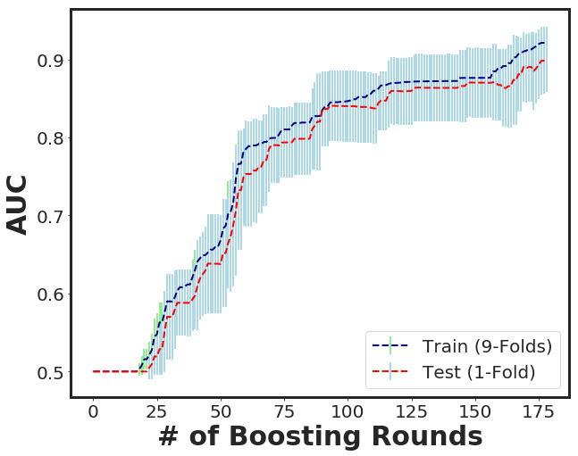
[178] train-auc:0.922025+0.00538528 test-auc:0.900192+0.0420388
*-*- Boosting Round = 178 -*-*- Train = 0.922 -*-*- Test = 0.9 -*-*
-*-*-*-*-*-*-* Train Started *-*-*-*-*-*-*-
[22:09:58] Tree method is selected to be 'hist', which uses a single updater grow_fast_histmaker.
_plot_xgboost_cv_score(cvr)
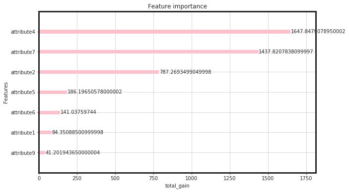
_plot_importance(bst, figsize=(10,6), importance_type = "total_gain")
Tree_explainer = shap.TreeExplainer(bst)
shap_Treevalues = Tree_explainer.shap_values(df_X)
shap.summary_plot(shap_Treevalues, df_X, plot_type = "bar", color = "pink", max_display = 10)
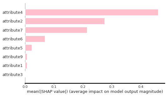
As seen, attribute3 has not played an important role through the feature selection process. Therefore, I dropped it and build the final model based on that.
df_pruned = df_X.drop(["attribute3"], axis = 1)
As seen, the total gain for attribute4, attirbute7, and attribute 2 are higher than the rest. This would say that, for linear models such as regulirized linear models including elastic net, these features will be pruned. Now, we can see, how these features perform:
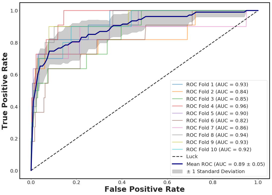
_plot_roc_nfolds_xgboost(df_pruned, Y)
test_size = 0.3
n_folds = 10
accuracy_score, roc_score, cv_roc_score, y_pred_prob, X_test, y_test, optimal_threshold = _clf_xgboost(df_pruned, Y, test_size, n_folds)
CI_neg, CI_pos = _ConfidenceInterval(roc_score, X_test.shape[0])
print(F"Accuracy for test size {test_size} = {accuracy_score:.5f}")
print(F"ROC for test size {test_size} = {roc_score:.3f}")
print(F"Mean ROC for {n_folds} folds CV = {cv_roc_score.mean():.3f}")
print(F"Confidence Interval Accuracy = [{CI_neg:.3f} , {CI_pos:.3f}]")
class_names = [0, 1]
#optimal threshold based on Youden Index
y_pred = (y_pred_prob[:,1] > optimal_threshold).astype(int)
# Compute confusion matrix
cnf_matrix = confusion_matrix(y_test, y_pred)
np.set_printoptions(precision=2)
# Plot normalized confusion matrix
plt.figure(figsize=(6,6))
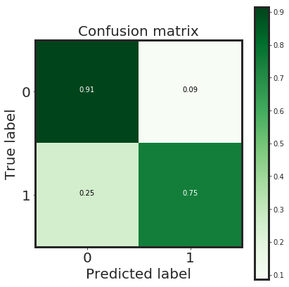
_plot_confusion_matrix(cnf_matrix, classes=class_names, normalize = True)
plt.show()
Accuracy for test size 0.3  = 0.99914
ROC for test size 0.3 = 0.890
Mean ROC for 10 folds CV = 0.896
Confidence Interval Accuracy = [0.887 , 0.893]
Normalized confusion matrix
[[0.91 0.09]
 [0.25 0.75]]
Discussion:
As seen, the xgboost approach showed a good performance in terms of classification of the individuals in terms of Failure and Non-failure. The classification problem is an imbalanced problem (prevalence < 1%). Therefore, the classification accuracy by itself cannot be trusted and the other classification metrics such as area under ROC curve and Precision-Recalls or F-1 score which are robust to imbalanced classes should be used. The other challenge is the size of the dataset. In fact, we are looking for a model that can be generalized to a larger population. In this regard, it is also better to report the classification error with a confidence interval at a statistical significance level. For instance, to have 95% significance, we can calculate the classification error from the following formula using the Z-score of 1.96:
$ConfidenceInterval = Score \pm 1.96 \times \sqrt{ \frac{Score \times (1 - Score)}{N}}$
For instance, for the approach , we have N= 37349 (30% of the data) individuals in the testing set (unseen individuals) with an AUC of 0.89 which is within the calculated 95% confidence interval. Now, we can add the prediction pribabilities for both class 0 and 1 to the test data.
X_test["pred_proba_class_0"] = pd.Series(y_pred_prob[:,0], index = X_test.index)
X_test["pred_proba_class_1"] = pd.Series(y_pred_prob[:,1], index = X_test.index)
print(F"Test Size = {X_test.shape}")
X_test.head()
Test Size = (37349, 9)
| attribute1 | attribute2 | attribute4 | attribute5 | attribute6 | attribute7 | attribute9 | pred_proba_class_0 | pred_proba_class_1 | |
|---|---|---|---|---|---|---|---|---|---|
| 22999 | 0.394775 | -0.073170 | -0.076004 | -0.202137 | -0.414557 | -0.039335 | -0.065047 | 0.999829 | 0.000171 |
| 26237 | -1.097957 | 0.844409 | -0.076004 | 0.613269 | -2.623549 | -0.039335 | -0.065047 | 0.997224 | 0.002776 |
| 123435 | -1.179217 | -0.073170 | -0.076004 | -0.515755 | 0.573101 | -0.039335 | -0.065047 | 0.999710 | 0.000290 |
| 120834 | 0.404221 | -0.073170 | -0.076004 | -0.515755 | 1.461849 | -0.039335 | -0.065047 | 0.999801 | 0.000199 |
| 31117 | 0.243279 | -0.073170 | -0.076004 | 1.428676 | 0.208837 | -0.039335 | -0.065047 | 0.999160 | 0.000840 |
Now we can repeat this process for N times (let’s do 100 times) and check the histograms of auc for 95% significance level.
_xgboost_auc_hist(df_pruned, Y, n_iterations = 100, alpha = 0.95)
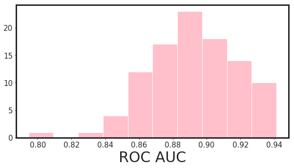
95.0% Significance Level - ROC AUC Confidence Interval= [0.849 , 0.934]
Note that, in this example I have chosen the hyper-parameters based on rule of thumb and my experience. However, for finalizing the model, an exhaustive GridSearch or Bayesian Optimization is needed. I have not done it here due to my short time to finish this project. However, for all of my model that went to production so far, I do use hyper-parameter tuning.
2nd Approach: Regularized Linear Model
# Ridge
alpha = 0.0

glmnet_model = _glmnet(df_X, Y, alpha = alpha)
_plot_glmnet_coeff_path(glmnet_model, df_X)
_plot_glmnet_cv_score(glmnet_model)
_df_glmnet_coeff_path(glmnet_model, df_X)
| Features | Coeffs | |
|---|---|---|
| 0 | attribute7 | 0.001592 |
| 1 | attribute4 | 0.000901 |
| 2 | attribute2 | 0.000707 |
| 3 | attribute5 | 0.000030 |
| 4 | attribute1 | 0.000027 |
| 5 | attribute9 | 0.000022 |
| 6 | attribute6 | -0.000007 |
| 7 | attribute3 | -0.000013 |
_glmnet_best_score_alpha(df_X, Y)
# Elastic-Net
alpha = 0.1
glmnet_model = _glmnet(df_X, Y, alpha = alpha)
_plot_glmnet_coeff_path(glmnet_model, df_X)
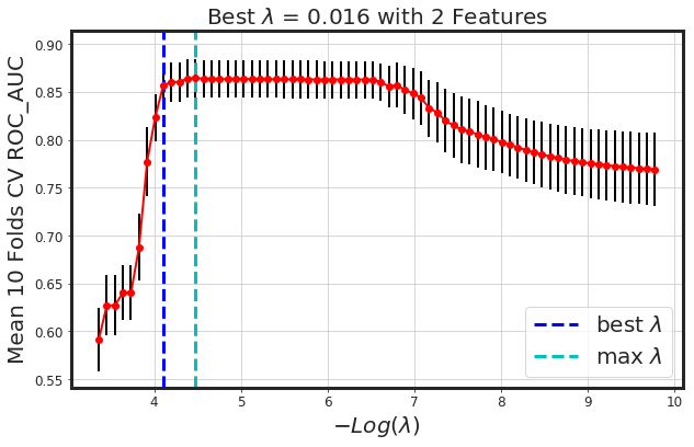
_plot_glmnet_cv_score(glmnet_model)
_df_glmnet_coeff_path(glmnet_model, df_X)
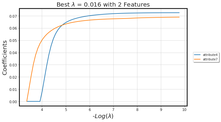
| Features | Coeffs | |
|---|---|---|
| 0 | attribute7 | 0.052871 |
| 1 | attribute4 | 0.018768 |
As seen, glmnet has added more bias to the model (we lost around 4% AUC). However, the model is way more simpler. Generally, both methods along with each other would result in a more generalized model.
Notes could be considered:
Other than, hyper parameter optimization (using grid search or bayesian optimization), I have not implemented any neural network models here that could be used as well (neural network without hyper-parameter optimizaiton is technically useless). Another thing that could be used is the time at event. For example, any useful information such as some specific day-of-the-month that failure happened can be engineered as a new feature (attribute). In addition to this, the device include 1169 unique values where failure happened for 106 of them.
g = df_raw.groupby("device").agg({"failure" : "mean"}).sort_values(by = ["failure"], ascending = False)
g = g.reset_index(level=["device"])
print(F"Number of groups with non-zero failure rate = {g[g['failure'] > 0].shape[0]}")
g.head(10)
Number of groups with non-zero failure rate = 106
| device | failure | |
|---|---|---|
| 0 | S1F0RRB1 | 0.200000 |
| 1 | S1F10E6M | 0.142857 |
| 2 | S1F11MB0 | 0.142857 |
| 3 | S1F0CTDN | 0.142857 |
| 4 | Z1F1AG5N | 0.111111 |
| 5 | W1F0PNA5 | 0.111111 |
| 6 | W1F13SRV | 0.076923 |
| 7 | W1F03DP4 | 0.071429 |
| 8 | W1F1230J | 0.071429 |
| 9 | W1F0T034 | 0.058824 |