Glass Identification

Introduction
Glass fragments are one of the most frequently used items in forensic science. In most of the crime scences such as house-breaking, even small fragments of the glass attached to the clothes of the person who is suspected would solve the problem. Even from small glass fragments, based on the elemntal composition and more importantly the refractive index, we can say where this fragment comes from. Does it come from a house window or car windshield or a beer bottle, and etc. In this regard, I have employed the “Glass Identification” dataset, published by Ian W Evett [1]. He worke several years as an operational forensic scientist.
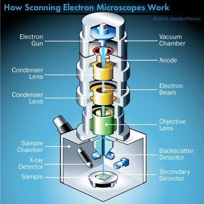
The most useful characteristics of glass for forensic purposes represents the refractive index (RI) which has a high precision even for small pieces. For even larger fragments, the elemental components can be obtained using a Scanning Electron Microscope. The data colleceted for 214 glass samples and were analyzed at the Home Office Forensic Science Laboratory, Birmingham.
First of all, we need to call the librarie that we would need in the future coding here:
import numpy as np
import pandas as pd
import matplotlib.pyplot as plt
import seaborn as sns
import matplotlib as mpl
from sklearn.preprocessing import scale
from pandas.tools.plotting import scatter_matrix
from sklearn.metrics import classification_report
from sklearn.multiclass import OneVsRestClassifier
from sklearn.svm import SVC
from sklearn.cross_validation import cross_val_score
from sklearn.cross_validation import cross_val_predict
from sklearn.model_selection import train_test_split
from keras.models import Sequential
from keras.layers import Dense
from keras.layers import Dropout
from keras.wrappers.scikit_learn import KerasClassifier
from sklearn.preprocessing import Imputer
from sklearn import preprocessing
from sklearn.preprocessing import OneHotEncoder
from sklearn.metrics import make_scorer
from sklearn.metrics import accuracy_score
from sklearn.model_selection import GridSearchCV
from sklearn.ensemble import GradientBoostingClassifier
from sklearn.tree import DecisionTreeClassifier
from sklearn.ensemble import RandomForestClassifier
from sklearn.linear_model import LogisticRegression
from sklearn.pipeline import Pipeline
from sklearn import linear_model
from tpot import TPOTClassifier
from matplotlib import pyplot
from IPython.display import Image
from math import cos, sin, atan
from sklearn import decomposition
import warnings
warnings.filterwarnings("ignore")
sns.set_style("ticks")
Now, let’s read the database into a dataframe.
Headers = ["RI" , "Na", "Mg", "Al", "Si", "K", "Ca", "Ba", "Fe", "Type"]
Data = pd.read_csv("../Data/Glass.txt" , sep = "," , names = Headers)
Here is the first 5 rows of the database.
Data.head(5)
| RI | Na | Mg | Al | Si | K | Ca | Ba | Fe | Type | |
|---|---|---|---|---|---|---|---|---|---|---|
| 1 | 1.52101 | 13.64 | 4.49 | 1.10 | 71.78 | 0.06 | 8.75 | 0.0 | 0.0 | 1 |
| 2 | 1.51761 | 13.89 | 3.60 | 1.36 | 72.73 | 0.48 | 7.83 | 0.0 | 0.0 | 1 |
| 3 | 1.51618 | 13.53 | 3.55 | 1.54 | 72.99 | 0.39 | 7.78 | 0.0 | 0.0 | 1 |
| 4 | 1.51766 | 13.21 | 3.69 | 1.29 | 72.61 | 0.57 | 8.22 | 0.0 | 0.0 | 1 |
| 5 | 1.51742 | 13.27 | 3.62 | 1.24 | 73.08 | 0.55 | 8.07 | 0.0 | 0.0 | 1 |
To describe the statistics of the database we have:
Data.describe()
| RI | Na | Mg | Al | Si | K | Ca | Ba | Fe | Type | |
|---|---|---|---|---|---|---|---|---|---|---|
| count | 214.000000 | 214.000000 | 214.000000 | 214.000000 | 214.000000 | 214.000000 | 214.000000 | 214.000000 | 214.000000 | 214.000000 |
| mean | 1.518365 | 13.407850 | 2.684533 | 1.444907 | 72.650935 | 0.497056 | 8.956963 | 0.175047 | 0.057009 | 2.780374 |
| std | 0.003037 | 0.816604 | 1.442408 | 0.499270 | 0.774546 | 0.652192 | 1.423153 | 0.497219 | 0.097439 | 2.103739 |
| min | 1.511150 | 10.730000 | 0.000000 | 0.290000 | 69.810000 | 0.000000 | 5.430000 | 0.000000 | 0.000000 | 1.000000 |
| 25% | 1.516523 | 12.907500 | 2.115000 | 1.190000 | 72.280000 | 0.122500 | 8.240000 | 0.000000 | 0.000000 | 1.000000 |
| 50% | 1.517680 | 13.300000 | 3.480000 | 1.360000 | 72.790000 | 0.555000 | 8.600000 | 0.000000 | 0.000000 | 2.000000 |
| 75% | 1.519157 | 13.825000 | 3.600000 | 1.630000 | 73.087500 | 0.610000 | 9.172500 | 0.000000 | 0.100000 | 3.000000 |
| max | 1.533930 | 17.380000 | 4.490000 | 3.500000 | 75.410000 | 6.210000 | 16.190000 | 3.150000 | 0.510000 | 7.000000 |
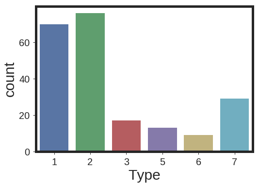
where RI is refractive index, Na is Sodium, Mg is Magnesium, Al is Aluminum, Si is Silicon, K is Potassium, Ca is Calcium, Ba is Barium, and Fe is Iron. Type would present the 6 different types of glass in the database including: 1) float processed building windows, 2) non float processed building windows, 3) float processed vehicle windows, 5) containers, 6) tableware, 7) headlamps.
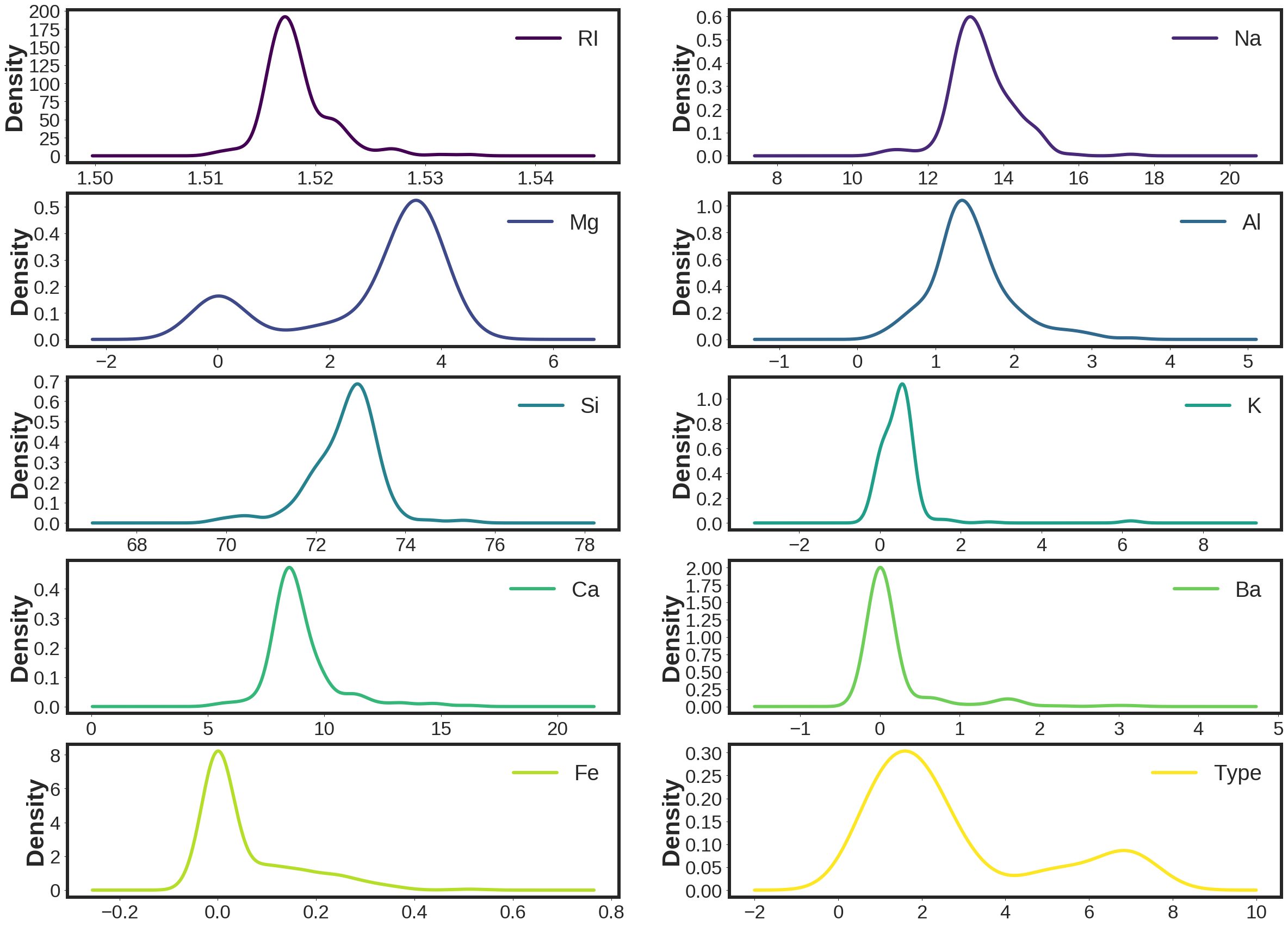
Now let’s try to visualize the database a little bit more:
Here is the density plots of the attributes of the database.
plt.figure()
mpl.rcParams['axes.linewidth'] = 6 #set the value globally
mpl.rcParams['legend.fontsize'] = 40 #set the value globally
Axes = Data.plot(kind='density',lw=6, subplots=True, layout=(5,2),figsize=(40, 30),
                 sharex = False ,sharey=False, legend=True , colormap = "viridis")
[plt.setp(item.yaxis.get_majorticklabels(), 'size', 35) for item in Axes.ravel()]
[plt.setp(item.xaxis.get_majorticklabels(), 'size', 35) for item in Axes.ravel()]
[plt.setp(item.yaxis.get_label(), 'size', 45) for item in Axes.ravel()]
[plt.setp(item.xaxis.get_label(), 'size', 45) for item in Axes.ravel()]
[plt.setp(item.yaxis.get_label(), 'weight', 'bold') for item in Axes.ravel()]
plt.show()
<matplotlib.figure.Figure at 0x7f59c6c85650>
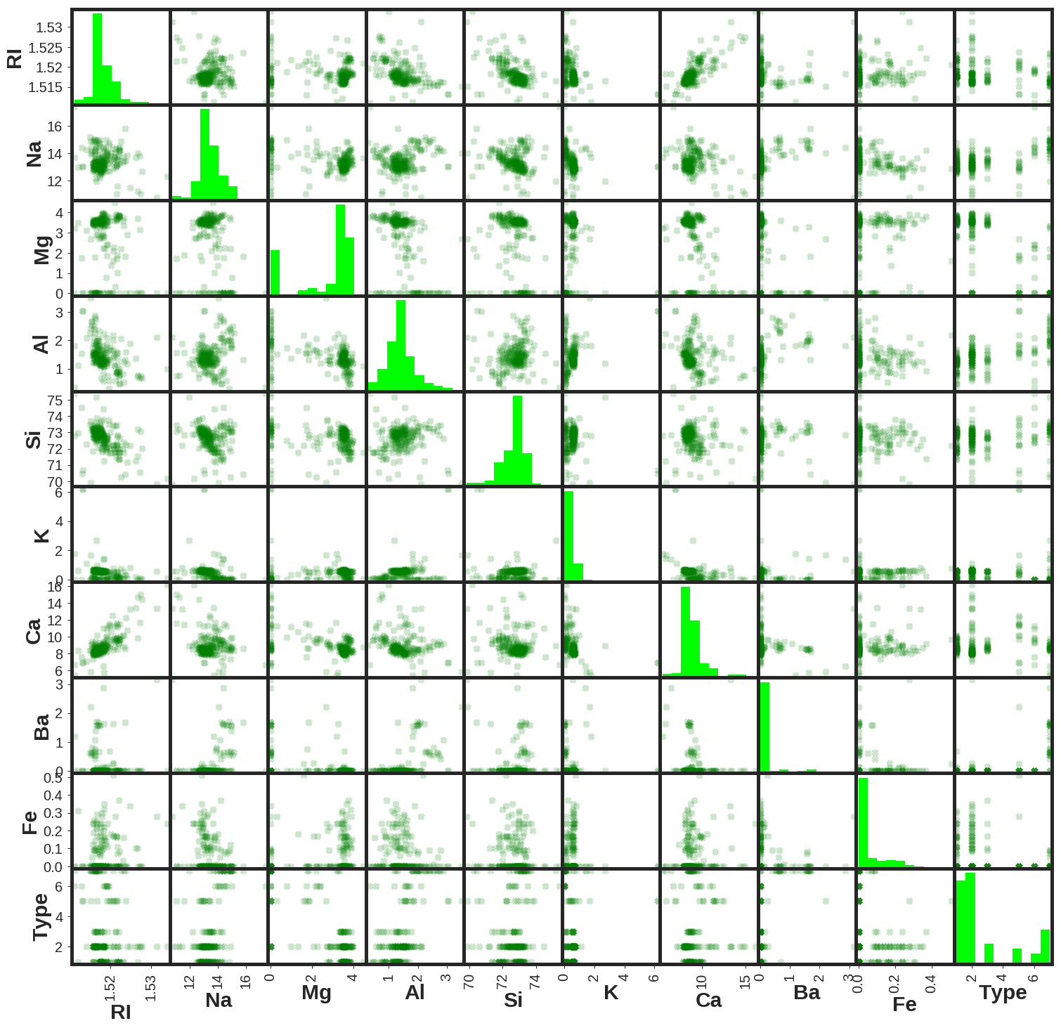
Here is the presentation of the scatter matrix of the database.
plt.figure()
mpl.rcParams['axes.linewidth'] = 5
Axes = scatter_matrix(Data , alpha=0.2, lw=5 ,c='g',marker='x',hist_kwds={'color':['lime']},figsize=(25, 25))
[plt.setp(item.yaxis.get_majorticklabels(), 'size', 20) for item in Axes.ravel()]
[plt.setp(item.xaxis.get_majorticklabels(), 'size', 20) for item in Axes.ravel()]
[plt.setp(item.yaxis.get_label(), 'size', 30) for item in Axes.ravel()]
[plt.setp(item.xaxis.get_label(), 'size', 30) for item in Axes.ravel()]
[plt.setp(item.xaxis.get_label(), 'weight', 'bold') for item in Axes.ravel()]
[plt.setp(item.yaxis.get_label(), 'weight', 'bold') for item in Axes.ravel()]
plt.show()
<matplotlib.figure.Figure at 0x7f59c6633250>
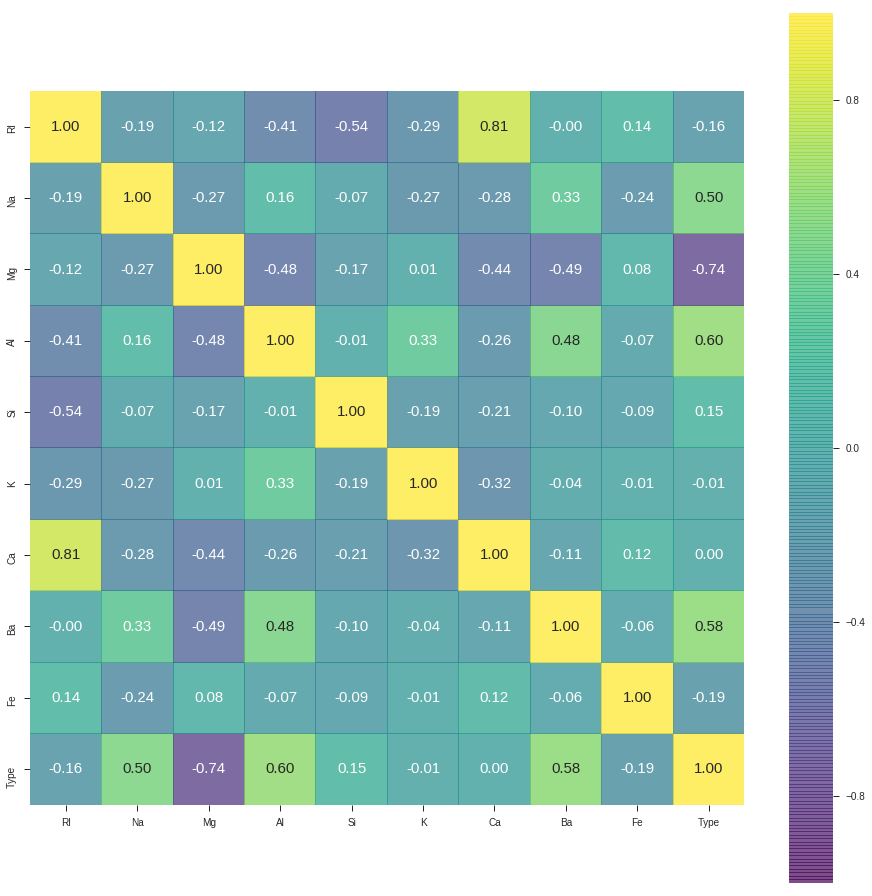
Here we can present the heatmap presentation of the data
corr = Data.corr()
plt.figure(figsize=(16,16))
sns.heatmap(corr, cbar = True,  square = True, annot=True, fmt= '.2f',annot_kws={'size': 15},
           xticklabels=Data.columns.values, yticklabels= Data.columns.values, alpha = 0.7,   cmap= 'viridis')
plt.show()
Here is the presentation of the counts for each class in the database
plt.rcParams["xtick.labelsize"] = 20
plt.rcParams["ytick.labelsize"] = 20
plt.rcParams["axes.labelsize"] = 30
sns.countplot( Data['Type']  , linewidth=5,  label='big')
plt.show()
Now, we need to put the features and labels into numpy arrays. In addition to this, I have used the standardized transformation on the data to have zero mean and units standard deviation.
Y = Data["Type"].values
del Data["Type"]
X = Data.values
X_scaled = scale(X)
Y = Y.astype(float)
It may be relevant to see how the data clusters look like. In this regard, I plotted the scatter plots of the data in different 2D surfaces.
plt.figure(figsize=(34 , 14))

plt.subplot(2 , 4, 1)
plt.scatter(X_scaled[:,0] , X_scaled[:,1] ,s = 70, c = Y, cmap = "viridis"  )
plt.legend(loc = 0)
plt.xlabel("RI")
plt.ylabel("Na")

plt.subplot(2 , 4, 2)
plt.scatter(X_scaled[:,0] , X_scaled[:,2] ,s = 70, c = Y, cmap = "viridis"  )
plt.legend(loc = 0)
plt.xlabel("RI")
plt.ylabel("Mg")

plt.subplot(2 , 4, 3)
plt.scatter(X_scaled[:,0] , X_scaled[:,3] ,s = 70, c = Y, cmap = "viridis"  )
plt.legend(loc = 0)
plt.xlabel("RI")
plt.ylabel("Al")

plt.subplot(2 , 4, 4)
plt.scatter(X_scaled[:,0] , X_scaled[:,4] ,s = 70, c = Y, cmap = "viridis"  )
plt.legend(loc = 0)
plt.xlabel("RI")
plt.ylabel("Si")

plt.subplot(2 , 4, 5)
plt.scatter(X_scaled[:,0] , X_scaled[:,5] ,s = 70, c = Y, cmap = "viridis"  )
plt.legend(loc = 0)
plt.xlabel("RI")
plt.ylabel("K")

plt.subplot(2 , 4, 6)
plt.scatter(X_scaled[:,0] , X_scaled[:,6] ,s = 70, c = Y, cmap = "viridis"  )
plt.legend(loc = 0)
plt.xlabel("RI")
plt.ylabel("Ca")

plt.subplot(2 , 4, 7)
plt.scatter(X_scaled[:,0] , X_scaled[:,7] ,s = 70, c = Y, cmap = "viridis"  )
plt.legend(loc = 0)
plt.xlabel("RI")
plt.ylabel("Ba")

plt.subplot(2 , 4, 8)
plt.scatter(X_scaled[:,0] , X_scaled[:,8] ,s = 70, c = Y, cmap = "viridis"  )
plt.legend(loc = 0)
plt.xlabel("RI")
plt.ylabel("Fe")

plt.show()
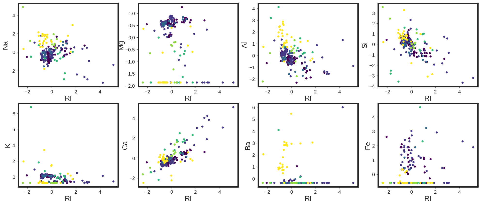
As shown, each color represents one of the classes out of six present class in this data base. It is also clear that, the classifiation is not trivial for this data base. To test it out, I have started with five different classifiers, including Logistic Regression, Support Vector Machine with Linear kernel, Support Vector Machine with Radial Basis Function Kernel, Random Forests, and GradientBoostingTrees using One versus Rest classifiers. In this regard, for each classifier, the class is fitted against all the other classes. In addition to its computational efficiency, one advantage of this approach is its interpretability. Since each class is represented by one and only one classifier, it is possible to gain knowledge about the class by inspecting its corresponding classifier. This is the most commonly used strategy for multiclass classification and is a fair default choice.
To do this, first we need to define the training and testing dataset. I have used 75% of the data as training set and 25% of the data as the testing set:
X_train, X_test, y_train, y_test = train_test_split(X_scaled, Y,train_size=0.75, test_size=0.25)
Classifier1: Logistic Regression
clf1 = OneVsRestClassifier(LogisticRegression(C =10 , random_state=1367))
clf1.fit(X_train , y_train)
y1 = clf1.predict(X_test)
print classification_report(y_test , y1)
print "Classification Accuracy = " + str(accuracy_score(y_test , y1))
             precision    recall  f1-score   support

        1.0       0.65      0.69      0.67        16
        2.0       0.62      0.59      0.60        22
        3.0       0.33      0.25      0.29         4
        5.0       0.50      0.67      0.57         3
        6.0       0.67      0.67      0.67         3
        7.0       1.00      1.00      1.00         6

avg / total       0.64      0.65      0.64        54

Classification Accuracy = 0.648148148148
Classifer2: Linear SVM
clf2 = OneVsRestClassifier(SVC(kernel='linear',C = 1,probability=True,random_state=1367))
clf2.fit(X_train , y_train)
y2 = clf2.predict(X_test)
print classification_report(y_test , y2)
print "Classification Accuracy = " + str(accuracy_score(y_test , y2))
             precision    recall  f1-score   support

        1.0       0.52      1.00      0.68        16
        2.0       0.71      0.23      0.34        22
        3.0       0.00      0.00      0.00         4
        5.0       0.40      0.67      0.50         3
        6.0       0.67      0.67      0.67         3
        7.0       0.86      1.00      0.92         6

avg / total       0.60      0.57      0.51        54

Classification Accuracy = 0.574074074074
Classifier3: RBF SVM
clf3 = OneVsRestClassifier(SVC(kernel='rbf',C = 100, gamma = 0.1, probability=True,random_state=1367))
clf3.fit(X_train , y_train)
y3 = clf3.predict(X_test)
print classification_report(y_test , y3)
print "Classification Accuracy = " + str(accuracy_score(y_test , y3))
             precision    recall  f1-score   support

        1.0       0.71      0.75      0.73        16
        2.0       0.67      0.64      0.65        22
        3.0       0.20      0.25      0.22         4
        5.0       0.50      0.67      0.57         3
        6.0       1.00      0.33      0.50         3
        7.0       1.00      1.00      1.00         6

avg / total       0.69      0.67      0.67        54

Classification Accuracy = 0.666666666667
Classifier4 : Random Forests
clf4 = OneVsRestClassifier(RandomForestClassifier(n_estimators=200 ,min_samples_split=2 ,
                                                  min_samples_leaf=5, n_jobs=-1,  random_state=1367))
clf4.fit(X_train , y_train)
y4 = clf4.predict(X_test)
print classification_report(y_test , y4)
print "Classification Accuracy = " + str(accuracy_score(y_test , y4))
             precision    recall  f1-score   support

        1.0       0.71      0.94      0.81        16
        2.0       0.76      0.86      0.81        22
        3.0       0.00      0.00      0.00         4
        5.0       1.00      0.33      0.50         3
        6.0       1.00      0.33      0.50         3
        7.0       1.00      1.00      1.00         6

avg / total       0.74      0.78      0.74        54

Classification Accuracy = 0.777777777778
Classifier5: Gradient Boosting
clf5 = OneVsRestClassifier(GradientBoostingClassifier(n_estimators=200 , random_state=1367))
clf5.fit(X_train , y_train)
y5 = clf5.predict(X_test)
print classification_report(y_test , y5)
print "Classification Accuracy = " + str(accuracy_score(y_test , y5))
             precision    recall  f1-score   support

        1.0       0.79      0.69      0.73        16
        2.0       0.71      0.77      0.74        22
        3.0       0.40      0.50      0.44         4
        5.0       0.50      0.67      0.57         3
        6.0       1.00      0.33      0.50         3
        7.0       1.00      1.00      1.00         6

avg / total       0.75      0.72      0.72        54

Classification Accuracy = 0.722222222222
As shown, by employing different classifiers we can improve the classification accuracy. But the question we need to answer is if the classification results can be trusted? Or is this the best classification method I can use for this database?
To answer the aforementioned questions, I have used Genetic Programming to find the best possible pipeline out of 100 possible pipelines in 100 generations. In addition to this , I have used 5-folds cross-validation to decrease the chanve of overfitting. At the end, the best pipeline will be printed out.
tpot = TPOTClassifier(generations=100, population_size=100,cv = 5, verbosity=2, n_jobs=-1 , random_state=1367)
tpot.fit(X_train, y_train)
print(tpot.score(X_test, y_test))
Optimization Progress:   2%|▏         | 200/10100 [01:13<2:25:27,  1.13pipeline/s]

Generation 1 - Current best internal CV score: 0.779934131606


Optimization Progress:   3%|▎         | 300/10100 [02:06<2:03:53,  1.32pipeline/s]

Generation 2 - Current best internal CV score: 0.779934131606


Optimization Progress:   4%|▍         | 400/10100 [02:59<2:09:52,  1.24pipeline/s]

Generation 3 - Current best internal CV score: 0.779934131606


Optimization Progress:   5%|▍         | 500/10100 [03:59<1:59:16,  1.34pipeline/s]

Generation 4 - Current best internal CV score: 0.779934131606


Optimization Progress:   6%|▌         | 600/10100 [05:06<1:42:36,  1.54pipeline/s]

Generation 5 - Current best internal CV score: 0.779934131606


Optimization Progress:   7%|▋         | 700/10100 [06:06<3:06:10,  1.19s/pipeline]

Generation 6 - Current best internal CV score: 0.78620749139


Optimization Progress:   8%|▊         | 800/10100 [07:10<1:38:25,  1.57pipeline/s]

Generation 7 - Current best internal CV score: 0.787133257591


Optimization Progress:   9%|▉         | 900/10100 [08:01<2:16:39,  1.12pipeline/s]

Generation 8 - Current best internal CV score: 0.817327035982


Optimization Progress:  10%|▉         | 1000/10100 [08:50<1:26:33,  1.75pipeline/s]

Generation 9 - Current best internal CV score: 0.817327035982


Optimization Progress:  11%|█         | 1100/10100 [09:49<2:13:24,  1.12pipeline/s]

Generation 10 - Current best internal CV score: 0.817327035982


Optimization Progress:  12%|█▏        | 1200/10100 [10:40<1:54:16,  1.30pipeline/s]

Generation 11 - Current best internal CV score: 0.829448248103


Optimization Progress:  13%|█▎        | 1300/10100 [11:27<1:00:17,  2.43pipeline/s]

Generation 12 - Current best internal CV score: 0.829448248103


Optimization Progress:  14%|█▍        | 1400/10100 [12:11<1:34:04,  1.54pipeline/s]

Generation 13 - Current best internal CV score: 0.829448248103


Optimization Progress:  15%|█▍        | 1500/10100 [13:02<1:09:30,  2.06pipeline/s]

Generation 14 - Current best internal CV score: 0.829448248103


Optimization Progress:  16%|█▌        | 1600/10100 [13:53<2:01:21,  1.17pipeline/s]

Generation 15 - Current best internal CV score: 0.829448248103


Optimization Progress:  17%|█▋        | 1700/10100 [14:45<1:12:40,  1.93pipeline/s]

Generation 16 - Current best internal CV score: 0.829448248103


Optimization Progress:  18%|█▊        | 1800/10100 [15:36<1:43:40,  1.33pipeline/s]

Generation 17 - Current best internal CV score: 0.829448248103


Optimization Progress:  19%|█▉        | 1900/10100 [16:32<1:39:04,  1.38pipeline/s]

Generation 18 - Current best internal CV score: 0.829448248103


Optimization Progress:  20%|█▉        | 2000/10100 [17:18<1:36:48,  1.39pipeline/s]

Generation 19 - Current best internal CV score: 0.829448248103


Optimization Progress:  21%|██        | 2100/10100 [18:04<1:17:34,  1.72pipeline/s]

Generation 20 - Current best internal CV score: 0.829448248103


Optimization Progress:  22%|██▏       | 2200/10100 [19:41<2:08:53,  1.02pipeline/s]

Generation 21 - Current best internal CV score: 0.829448248103


Optimization Progress:  23%|██▎       | 2300/10100 [21:38<2:18:34,  1.07s/pipeline]

Generation 22 - Current best internal CV score: 0.829448248103


Optimization Progress:  24%|██▍       | 2400/10100 [22:28<1:09:27,  1.85pipeline/s]

Generation 23 - Current best internal CV score: 0.829448248103


Optimization Progress:  25%|██▍       | 2500/10100 [23:23<1:10:34,  1.79pipeline/s]

Generation 24 - Current best internal CV score: 0.829448248103


Optimization Progress:  26%|██▌       | 2600/10100 [24:32<1:39:32,  1.26pipeline/s]

Generation 25 - Current best internal CV score: 0.829448248103


Optimization Progress:  27%|██▋       | 2700/10100 [25:43<1:50:25,  1.12pipeline/s]

Generation 26 - Current best internal CV score: 0.829448248103


Optimization Progress:  28%|██▊       | 2800/10100 [26:49<1:05:59,  1.84pipeline/s]

Generation 27 - Current best internal CV score: 0.830284193766


Optimization Progress:  29%|██▊       | 2900/10100 [28:43<1:46:33,  1.13pipeline/s]

Generation 28 - Current best internal CV score: 0.830284193766


Optimization Progress:  30%|██▉       | 3000/10100 [29:49<1:56:22,  1.02pipeline/s]

Generation 29 - Current best internal CV score: 0.830284193766


Optimization Progress:  31%|███       | 3100/10100 [30:42<1:30:50,  1.28pipeline/s]

Generation 30 - Current best internal CV score: 0.830284193766


Optimization Progress:  32%|███▏      | 3200/10100 [31:30<59:28,  1.93pipeline/s]

Generation 31 - Current best internal CV score: 0.830284193766


Optimization Progress:  33%|███▎      | 3300/10100 [32:18<1:07:19,  1.68pipeline/s]

Generation 32 - Current best internal CV score: 0.830284193766


Optimization Progress:  34%|███▎      | 3400/10100 [33:13<1:28:52,  1.26pipeline/s]

Generation 33 - Current best internal CV score: 0.830284193766


Optimization Progress:  35%|███▍      | 3500/10100 [34:10<1:03:22,  1.74pipeline/s]

Generation 34 - Current best internal CV score: 0.830284193766


Optimization Progress:  36%|███▌      | 3600/10100 [35:00<1:26:16,  1.26pipeline/s]

Generation 35 - Current best internal CV score: 0.830284193766


Optimization Progress:  37%|███▋      | 3700/10100 [36:07<1:03:03,  1.69pipeline/s]

Generation 36 - Current best internal CV score: 0.830284193766


Optimization Progress:  38%|███▊      | 3800/10100 [37:00<1:09:26,  1.51pipeline/s]

Generation 37 - Current best internal CV score: 0.835899861006


Optimization Progress:  39%|███▊      | 3900/10100 [37:57<1:19:30,  1.30pipeline/s]

Generation 38 - Current best internal CV score: 0.835899861006


Optimization Progress:  40%|███▉      | 4000/10100 [38:46<1:03:35,  1.60pipeline/s]

Generation 39 - Current best internal CV score: 0.835899861006


Optimization Progress:  41%|████      | 4100/10100 [40:48<1:44:51,  1.05s/pipeline]

Generation 40 - Current best internal CV score: 0.835899861006


Optimization Progress:  42%|████▏     | 4200/10100 [41:52<1:05:29,  1.50pipeline/s]

Generation 41 - Current best internal CV score: 0.835899861006


Optimization Progress:  43%|████▎     | 4300/10100 [42:34<58:18,  1.66pipeline/s]

Generation 42 - Current best internal CV score: 0.835899861006


Optimization Progress:  44%|████▎     | 4400/10100 [45:33<3:40:53,  2.33s/pipeline]

Generation 43 - Current best internal CV score: 0.835899861006


Optimization Progress:  45%|████▍     | 4500/10100 [46:30<1:12:16,  1.29pipeline/s]

Generation 44 - Current best internal CV score: 0.835899861006


Optimization Progress:  46%|████▌     | 4600/10100 [47:23<51:03,  1.80pipeline/s]

Generation 45 - Current best internal CV score: 0.835899861006


Optimization Progress:  47%|████▋     | 4700/10100 [48:17<1:06:48,  1.35pipeline/s]

Generation 46 - Current best internal CV score: 0.835899861006


Optimization Progress:  48%|████▊     | 4800/10100 [49:00<51:56,  1.70pipeline/s]

Generation 47 - Current best internal CV score: 0.835899861006


Optimization Progress:  49%|████▊     | 4900/10100 [49:46<38:56,  2.23pipeline/s]

Generation 48 - Current best internal CV score: 0.835899861006


Optimization Progress:  50%|████▉     | 5000/10100 [50:23<32:43,  2.60pipeline/s]

Generation 49 - Current best internal CV score: 0.835899861006


Optimization Progress:  50%|█████     | 5100/10100 [51:00<41:42,  2.00pipeline/s]

Generation 50 - Current best internal CV score: 0.835899861006


Optimization Progress:  51%|█████▏    | 5200/10100 [51:42<21:39,  3.77pipeline/s]

Generation 51 - Current best internal CV score: 0.835899861006


Optimization Progress:  52%|█████▏    | 5300/10100 [52:32<53:48,  1.49pipeline/s]

Generation 52 - Current best internal CV score: 0.835899861006


Optimization Progress:  53%|█████▎    | 5400/10100 [53:12<37:17,  2.10pipeline/s]

Generation 53 - Current best internal CV score: 0.835899861006


Optimization Progress:  54%|█████▍    | 5500/10100 [53:48<28:25,  2.70pipeline/s]

Generation 54 - Current best internal CV score: 0.835899861006


Optimization Progress:  55%|█████▌    | 5600/10100 [54:28<31:44,  2.36pipeline/s]

Generation 55 - Current best internal CV score: 0.835899861006


Optimization Progress:  56%|█████▋    | 5700/10100 [55:14<28:09,  2.60pipeline/s]

Generation 56 - Current best internal CV score: 0.835899861006


Optimization Progress:  57%|█████▋    | 5800/10100 [55:50<30:27,  2.35pipeline/s]

Generation 57 - Current best internal CV score: 0.835899861006


Optimization Progress:  58%|█████▊    | 5900/10100 [56:35<24:21,  2.87pipeline/s]

Generation 58 - Current best internal CV score: 0.835899861006


Optimization Progress:  59%|█████▉    | 6000/10100 [57:15<21:08,  3.23pipeline/s]

Generation 59 - Current best internal CV score: 0.835899861006


Optimization Progress:  60%|██████    | 6100/10100 [57:53<26:59,  2.47pipeline/s]

Generation 60 - Current best internal CV score: 0.835899861006


Optimization Progress:  61%|██████▏   | 6200/10100 [58:28<28:13,  2.30pipeline/s]

Generation 61 - Current best internal CV score: 0.835899861006


Optimization Progress:  62%|██████▏   | 6300/10100 [59:05<19:14,  3.29pipeline/s]

Generation 62 - Current best internal CV score: 0.835899861006


Optimization Progress:  63%|██████▎   | 6400/10100 [59:42<27:28,  2.24pipeline/s]

Generation 63 - Current best internal CV score: 0.835899861006


Optimization Progress:  64%|██████▍   | 6500/10100 [1:00:38<22:06,  2.71pipeline/s]

Generation 64 - Current best internal CV score: 0.835899861006


Optimization Progress:  65%|██████▌   | 6600/10100 [1:01:26<26:01,  2.24pipeline/s]

Generation 65 - Current best internal CV score: 0.835899861006


Optimization Progress:  66%|██████▋   | 6700/10100 [1:02:13<28:39,  1.98pipeline/s]

Generation 66 - Current best internal CV score: 0.835899861006


Optimization Progress:  67%|██████▋   | 6800/10100 [1:02:47<24:42,  2.23pipeline/s]

Generation 67 - Current best internal CV score: 0.835899861006


Optimization Progress:  68%|██████▊   | 6900/10100 [1:03:24<20:01,  2.66pipeline/s]

Generation 68 - Current best internal CV score: 0.835899861006


Optimization Progress:  69%|██████▉   | 7000/10100 [1:04:04<22:31,  2.29pipeline/s]

Generation 69 - Current best internal CV score: 0.835899861006


Optimization Progress:  70%|███████   | 7100/10100 [1:04:42<15:07,  3.31pipeline/s]

Generation 70 - Current best internal CV score: 0.835899861006


Optimization Progress:  71%|███████▏  | 7200/10100 [1:05:15<12:14,  3.95pipeline/s]

Generation 71 - Current best internal CV score: 0.835899861006


Optimization Progress:  72%|███████▏  | 7300/10100 [1:05:49<17:56,  2.60pipeline/s]

Generation 72 - Current best internal CV score: 0.835899861006


Optimization Progress:  73%|███████▎  | 7400/10100 [1:06:24<20:29,  2.20pipeline/s]

Generation 73 - Current best internal CV score: 0.835899861006


Optimization Progress:  74%|███████▍  | 7500/10100 [1:07:18<12:29,  3.47pipeline/s]

Generation 74 - Current best internal CV score: 0.835899861006


Optimization Progress:  75%|███████▌  | 7600/10100 [1:07:57<17:58,  2.32pipeline/s]

Generation 75 - Current best internal CV score: 0.835899861006


Optimization Progress:  76%|███████▌  | 7700/10100 [1:08:41<13:27,  2.97pipeline/s]

Generation 76 - Current best internal CV score: 0.835899861006


Optimization Progress:  77%|███████▋  | 7800/10100 [1:09:18<15:08,  2.53pipeline/s]

Generation 77 - Current best internal CV score: 0.835899861006


Optimization Progress:  78%|███████▊  | 7900/10100 [1:09:54<09:56,  3.69pipeline/s]

Generation 78 - Current best internal CV score: 0.835899861006


Optimization Progress:  79%|███████▉  | 8000/10100 [1:10:30<13:36,  2.57pipeline/s]

Generation 79 - Current best internal CV score: 0.835899861006


Optimization Progress:  80%|████████  | 8100/10100 [1:11:08<13:40,  2.44pipeline/s]

Generation 80 - Current best internal CV score: 0.835899861006


Optimization Progress:  81%|████████  | 8200/10100 [1:11:45<11:49,  2.68pipeline/s]

Generation 81 - Current best internal CV score: 0.835899861006


Optimization Progress:  82%|████████▏ | 8300/10100 [1:12:27<16:25,  1.83pipeline/s]

Generation 82 - Current best internal CV score: 0.835899861006


Optimization Progress:  83%|████████▎ | 8400/10100 [1:13:04<10:59,  2.58pipeline/s]

Generation 83 - Current best internal CV score: 0.835899861006


Optimization Progress:  84%|████████▍ | 8500/10100 [1:13:52<14:21,  1.86pipeline/s]

Generation 84 - Current best internal CV score: 0.835899861006


Optimization Progress:  85%|████████▌ | 8600/10100 [1:14:30<11:31,  2.17pipeline/s]

Generation 85 - Current best internal CV score: 0.835899861006


Optimization Progress:  86%|████████▌ | 8700/10100 [1:15:21<14:41,  1.59pipeline/s]

Generation 86 - Current best internal CV score: 0.835899861006


Optimization Progress:  87%|████████▋ | 8800/10100 [1:16:00<07:10,  3.02pipeline/s]

Generation 87 - Current best internal CV score: 0.835899861006


Optimization Progress:  88%|████████▊ | 8900/10100 [1:16:34<05:01,  3.98pipeline/s]

Generation 88 - Current best internal CV score: 0.835899861006


Optimization Progress:  89%|████████▉ | 9000/10100 [1:17:18<05:51,  3.13pipeline/s]

Generation 89 - Current best internal CV score: 0.835899861006


Optimization Progress:  90%|█████████ | 9100/10100 [1:18:00<05:28,  3.04pipeline/s]

Generation 90 - Current best internal CV score: 0.835899861006


Optimization Progress:  91%|█████████ | 9200/10100 [1:18:42<04:25,  3.39pipeline/s]

Generation 91 - Current best internal CV score: 0.835899861006


Optimization Progress:  92%|█████████▏| 9300/10100 [1:19:19<03:29,  3.81pipeline/s]

Generation 92 - Current best internal CV score: 0.835899861006


Optimization Progress:  93%|█████████▎| 9400/10100 [1:19:56<04:35,  2.54pipeline/s]

Generation 93 - Current best internal CV score: 0.835899861006


Optimization Progress:  94%|█████████▍| 9500/10100 [1:21:42<06:22,  1.57pipeline/s]

Generation 94 - Current best internal CV score: 0.835899861006


Optimization Progress:  95%|█████████▌| 9600/10100 [1:22:37<05:31,  1.51pipeline/s]

Generation 95 - Current best internal CV score: 0.835899861006


Optimization Progress:  96%|█████████▌| 9700/10100 [1:23:11<02:41,  2.47pipeline/s]

Generation 96 - Current best internal CV score: 0.835899861006


Optimization Progress:  97%|█████████▋| 9800/10100 [1:23:56<02:30,  1.99pipeline/s]

Generation 97 - Current best internal CV score: 0.835899861006


Optimization Progress:  98%|█████████▊| 9900/10100 [1:24:51<01:53,  1.76pipeline/s]

Generation 98 - Current best internal CV score: 0.835899861006


Optimization Progress:  99%|█████████▉| 10000/10100 [1:25:39<01:08,  1.46pipeline/s]

Generation 99 - Current best internal CV score: 0.835899861006


Generation 100 - Current best internal CV score: 0.835899861006

Best pipeline: GradientBoostingClassifier(GaussianNB(PolynomialFeatures(MaxAbsScaler(VarianceThreshold(LogisticRegression(input_matrix, C=0.01, dual=False, penalty=l2), threshold=0.75)), degree=2, include_bias=False, interaction_only=False)), learning_rate=0.1, max_depth=3, max_features=0.35, min_samples_leaf=8, min_samples_split=17, n_estimators=100, subsample=0.65)
0.814814814815
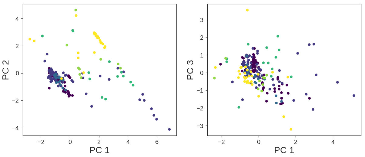
The other solution would be transforming the dataset to another subspace employing Principal Component Analysis. In this regard, I have designed a pipeline to determine the numbers of components that are necessary for the best classification.
pca = decomposition.PCA()
X_pca = pca.fit_transform(X)
plt.rcParams["xtick.labelsize"] = 20
plt.rcParams["ytick.labelsize"] = 20
plt.rcParams["axes.labelsize"] = 30
plt.figure(figsize=(20 , 8))

plt.subplot(1 , 2, 1)
plt.scatter(X_pca[:,0] , X_pca[:,1] ,s = 70, c = Y, cmap = "viridis"  )
plt.legend(loc = 0)
plt.xlabel("PC 1")
plt.ylabel("PC 2")

plt.subplot(1 , 2, 2)
plt.scatter(X_scaled[:,0] , X_pca[:,2] ,s = 70, c = Y, cmap = "viridis"  )
plt.legend(loc = 0)
plt.xlabel("PC 1")
plt.ylabel("PC 3")

plt.show()
PCA + Logistic Regression
logistic = linear_model.LogisticRegression()
pca = decomposition.PCA()
pipe = Pipeline(steps=[('pca', pca), ('logistic', logistic)])
pca.fit(X)
plt.figure( figsize=(8, 6))
plt.axes([.2, .2, .7, .7])
plt.plot(pca.explained_variance_, linewidth=2, color = "green")
plt.axis('tight')
plt.xlabel('# of PCs')
plt.xticks(range(1,10))
plt.ylabel('Explained Variance')

n_components = range(1,10)
Cs = np.logspace(-4, 4, 3)
estimator = GridSearchCV(pipe,dict(pca__n_components=n_components,logistic__C=Cs))
estimator.fit(X, Y)

plt.axvline(estimator.best_estimator_.named_steps['pca'].n_components,
            linestyle=':', color = "k", label='Best # of PCs')
plt.legend(loc = 0 ,prop=dict(size=15))
plt.show()
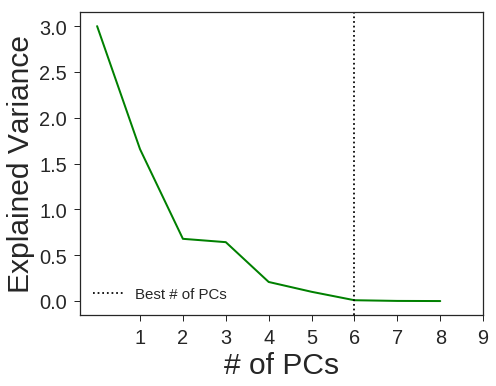
pca = decomposition.PCA(n_components=6, svd_solver='full', random_state=1367)
X_pca = pca.fit_transform(X)
X_train, X_test, y_train, y_test = train_test_split(X_pca, Y,train_size=0.75, test_size=0.25 , random_state = 1367)
clf1.fit(X_train , y_train)
y1 = clf1.predict(X_test)
print classification_report(y_test , y1)
print "Classification Accuracy = " + str(accuracy_score(y_test , y1))
             precision    recall  f1-score   support

        1.0       0.84      0.80      0.82        20
        2.0       0.62      0.83      0.71        18
        3.0       0.00      0.00      0.00         4
        5.0       0.00      0.00      0.00         2
        6.0       0.67      1.00      0.80         2
        7.0       1.00      0.88      0.93         8

avg / total       0.69      0.74      0.71        54

Classification Accuracy = 0.740740740741
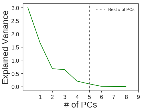
PCA + Linear SVM
svm = SVC(kernel='linear',probability=True,random_state=1367)
pca = decomposition.PCA()
pipe = Pipeline(steps=[('pca', pca), ('svm', svm)])
pca.fit(X)
plt.figure( figsize=(8, 6))
plt.axes([.2, .2, .7, .7])
plt.plot(pca.explained_variance_, linewidth=2, color = "green")
plt.axis('tight')
plt.xlabel('# of PCs')
plt.xticks(range(1,10))
plt.ylabel('Explained Variance')

n_components = range(1,10)
Cs = [1 , 10 , 100]
estimator = GridSearchCV(pipe,dict(pca__n_components=n_components,svm__C=Cs))
estimator.fit(X, Y)

plt.axvline(estimator.best_estimator_.named_steps['pca'].n_components,
            linestyle=':', color = "k", label='Best # of PCs')
plt.legend(loc = 0 ,prop=dict(size=15))
plt.show()

pca = decomposition.PCA(n_components=5, svd_solver='full', random_state=1367)
X_pca = pca.fit_transform(X)
X_train, X_test, y_train, y_test = train_test_split(X_pca, Y,train_size=0.75, test_size=0.25 , random_state = 1367)
clf2.fit(X_train , y_train)
y2 = clf2.predict(X_test)
print classification_report(y_test , y2)
print "Classification Accuracy = " + str(accuracy_score(y_test , y2))
             precision    recall  f1-score   support

        1.0       0.58      0.95      0.72        20
        2.0       0.67      0.22      0.33        18
        3.0       0.00      0.00      0.00         4
        5.0       0.40      1.00      0.57         2
        6.0       0.50      0.50      0.50         2
        7.0       1.00      0.88      0.93         8

avg / total       0.62      0.61      0.55        54

Classification Accuracy = 0.611111111111
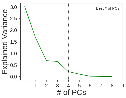
PCA + RBF SVM
svm = SVC(kernel='rbf',probability=True,random_state=1367)
pca = decomposition.PCA()
pipe = Pipeline(steps=[('pca', pca), ('svm', svm)])
pca.fit(X)
plt.figure( figsize=(8, 6))
plt.axes([.2, .2, .7, .7])
plt.plot(pca.explained_variance_, linewidth=2, color = "green")
plt.axis('tight')
plt.xlabel('# of PCs')
plt.xticks(range(1,10))
plt.ylabel('Explained Variance')

n_components = range(1,10)
Cs = [1 , 10 , 100]
Gammas = [0.001 , 0.01, 0.1 , 1]
estimator = GridSearchCV(pipe,dict(pca__n_components=n_components,svm__C=Cs,svm__gamma=Gammas))
estimator.fit(X, Y)

plt.axvline(estimator.best_estimator_.named_steps['pca'].n_components,
            linestyle=':', color = "k", label='Best # of PCs')
plt.legend(loc = 0 ,prop=dict(size=15))
plt.show()

pca = decomposition.PCA(n_components=4, svd_solver='full', random_state=1367)
X_pca = pca.fit_transform(X)
X_train, X_test, y_train, y_test = train_test_split(X_pca, Y,train_size=0.75, test_size=0.25 , random_state = 1367)
clf3.fit(X_train , y_train)
y3 = clf3.predict(X_test)
print classification_report(y_test , y3)
print "Classification Accuracy = " + str(accuracy_score(y_test , y3))
             precision    recall  f1-score   support

        1.0       0.73      0.80      0.76        20
        2.0       0.63      0.67      0.65        18
        3.0       0.00      0.00      0.00         4
        5.0       0.00      0.00      0.00         2
        6.0       0.50      1.00      0.67         2
        7.0       0.86      0.75      0.80         8

avg / total       0.63      0.67      0.64        54

Classification Accuracy = 0.666666666667
PCA + Random Forests
rf = RandomForestClassifier(random_state=1367)
pca = decomposition.PCA()
pipe = Pipeline(steps=[('pca', pca), ('rf', rf)])
pca.fit(X)
plt.figure( figsize=(8, 6))
plt.axes([.2, .2, .7, .7])
plt.plot(pca.explained_variance_, linewidth=2, color = "green")
plt.axis('tight')
plt.xlabel('# of PCs')
plt.xticks(range(1,10))
plt.ylabel('Explained Variance')

n_components = range(1,10)
trees = [30]

estimator = GridSearchCV(pipe,dict(pca__n_components=n_components,rf__n_estimators=trees))
estimator.fit(X, Y)

plt.axvline(estimator.best_estimator_.named_steps['pca'].n_components,
            linestyle=':', color = "k", label='Best # of PCs')
plt.legend(loc = 0 ,prop=dict(size=15))
plt.show()
clf4 = OneVsRestClassifier(RandomForestClassifier(n_estimators=40 ,min_samples_split=2 ,
                                                  min_samples_leaf=5, n_jobs=-1,  random_state=1367))
pca = decomposition.PCA(n_components=5, svd_solver='full', random_state=1367)
X_pca = pca.fit_transform(X)
X_train, X_test, y_train, y_test = train_test_split(X_pca, Y,train_size=0.75, test_size=0.25 , random_state = 1367)
clf4.fit(X_train , y_train)
y4 = clf4.predict(X_test)
print classification_report(y_test , y4)
print "Classification Accuracy = " + str(accuracy_score(y_test , y4))
             precision    recall  f1-score   support

        1.0       0.85      0.85      0.85        20
        2.0       0.75      0.83      0.79        18
        3.0       0.33      0.25      0.29         4
        5.0       0.00      0.00      0.00         2
        6.0       0.50      0.50      0.50         2
        7.0       1.00      1.00      1.00         8

avg / total       0.76      0.78      0.77        54

Classification Accuracy = 0.777777777778
gb = GradientBoostingClassifier(random_state=1367)
pca = decomposition.PCA()
pipe = Pipeline(steps=[('pca', pca), ('gb', gb)])
pca.fit(X)
plt.figure( figsize=(8, 6))
plt.axes([.2, .2, .7, .7])
plt.plot(pca.explained_variance_, linewidth=2, color = "green")
plt.axis('tight')
plt.xlabel('# of PCs')
plt.xticks(range(1,10))
plt.ylabel('Explained Variance')

n_components = range(1,10)
trees = [10]

estimator = GridSearchCV(pipe,dict(pca__n_components=n_components,gb__n_estimators=trees))
estimator.fit(X, Y)

plt.axvline(estimator.best_estimator_.named_steps['pca'].n_components,
            linestyle=':', color = "k", label='Best # of PCs')
plt.legend(loc = 0 ,prop=dict(size=15))
plt.show()
clf5 = OneVsRestClassifier(GradientBoostingClassifier(n_estimators=20 ,min_samples_leaf= 5 ,min_samples_split=50,
                                                      max_depth= 7 ,random_state=1367))
pca = decomposition.PCA(n_components=4, svd_solver='full', random_state=1367)
X_pca = pca.fit_transform(X)
X_train, X_test, y_train, y_test = train_test_split(X_pca, Y,train_size=0.75, test_size=0.25 , random_state = 1367)
clf5.fit(X_train , y_train)
y5 = clf5.predict(X_test)
print classification_report(y_test , y5)
print "Classification Accuracy = " + str(accuracy_score(y_test , y5))
             precision    recall  f1-score   support

        1.0       0.81      0.65      0.72        20
        2.0       0.68      0.83      0.75        18
        3.0       0.40      0.50      0.44         4
        5.0       0.00      0.00      0.00         2
        6.0       1.00      0.50      0.67         2
        7.0       1.00      0.88      0.93         8

avg / total       0.74      0.70      0.71        54

Classification Accuracy = 0.703703703704
To improve the classification accuracy, I decided to employ neural networks. Find below the architecture of this neural network:
class Neuron():
    def __init__(self, x, y):
        self.x = x
        self.y = y

    def draw(self, neuron_radius):
        circle = pyplot.Circle((self.x, self.y), radius=neuron_radius, color = "black", fill=True)
        pyplot.gca().add_patch(circle)


class Layer():
    def __init__(self, network, number_of_neurons, number_of_neurons_in_widest_layer):
        self.vertical_distance_between_layers = 60
        self.horizontal_distance_between_neurons = 20
        self.neuron_radius = 6
        self.number_of_neurons_in_widest_layer = number_of_neurons_in_widest_layer
        self.previous_layer = self.__get_previous_layer(network)
        self.y = self.__calculate_layer_y_position()
        self.neurons = self.__intialise_neurons(number_of_neurons)

    def __intialise_neurons(self, number_of_neurons):
        neurons = []
        x = self.__calculate_left_margin_so_layer_is_centered(number_of_neurons)
        for iteration in xrange(number_of_neurons):
            neuron = Neuron(x, self.y)
            neurons.append(neuron)
            x += self.horizontal_distance_between_neurons
        return neurons

    def __calculate_left_margin_so_layer_is_centered(self, number_of_neurons):
        return self.horizontal_distance_between_neurons*(self.number_of_neurons_in_widest_layer-number_of_neurons)/2

    def __calculate_layer_y_position(self):
        if self.previous_layer:
            return self.previous_layer.y + self.vertical_distance_between_layers
        else:
            return 0

    def __get_previous_layer(self, network):
        if len(network.layers) > 0:
            return network.layers[-1]
        else:
            return None

    def __line_between_two_neurons(self, neuron1, neuron2):
        angle = atan((neuron2.x - neuron1.x) / float(neuron2.y - neuron1.y))
        x_adjustment = self.neuron_radius * sin(angle)
        y_adjustment = self.neuron_radius * cos(angle)
        line = pyplot.Line2D((neuron1.x - x_adjustment, neuron2.x + x_adjustment),
                             (neuron1.y - y_adjustment, neuron2.y + y_adjustment) , color = "darkorange")
        pyplot.gca().add_line(line)

    def draw(self, layerType=0):
        for neuron in self.neurons:
            neuron.draw( self.neuron_radius )
            if self.previous_layer:
                for previous_layer_neuron in self.previous_layer.neurons:
                    self.__line_between_two_neurons(neuron, previous_layer_neuron)
        # write Text
        x_text = self.number_of_neurons_in_widest_layer * self.horizontal_distance_between_neurons
        if layerType == 0:
            pyplot.text(x_text, self.y, 'Input Layer', fontsize = 12)
        elif layerType == -1:
            pyplot.text(x_text, self.y, 'Output Layer', fontsize = 12)
        else:
            pyplot.text(x_text, self.y, 'Hidden Layer '+str(layerType), fontsize = 12)

class NeuralNetwork():
    def __init__(self, number_of_neurons_in_widest_layer):
        self.number_of_neurons_in_widest_layer = number_of_neurons_in_widest_layer
        self.layers = []
        self.layertype = 0

    def add_layer(self, number_of_neurons ):
        layer = Layer(self, number_of_neurons, self.number_of_neurons_in_widest_layer)
        self.layers.append(layer)

    def draw(self):
        pyplot.figure()
        for i in range( len(self.layers) ):
            layer = self.layers[i]
            if i == len(self.layers)-1:
                i = -1
            layer.draw( i )
        pyplot.axis('scaled')
        pyplot.axis('off')
        pyplot.title( 'Neural Network Architecture for Glass Data', fontsize=15 )
        pyplot.show()

class DrawNN():
    def __init__( self, neural_network ):
        self.neural_network = neural_network

    def draw( self ):
        widest_layer = max( self.neural_network )
        network = NeuralNetwork( widest_layer )
        for l in self.neural_network:
            network.add_layer(l)
        network.draw()

network = DrawNN( [9,8,7,6] )
network.draw()
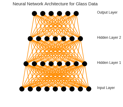
As shown, our model includes six different layers with 9, 8, 7, and 6 neurons in them respectively. For each layer a linear rectify with a dropout of 0.5 was employed. The activation function for the last layer has been set to softmax. To build this model with 6 different classes, we need to change the output labels into a matrix of 6 columns (each for each class) using one-hot-encoder:
YY = np.zeros((len(Y) , 1))
YY[:,0] = Y
enc = OneHotEncoder(sparse = False , handle_unknown='error')
enc.fit(YY)
Y_transformed = enc.transform(YY)
print "The Shape of the Transformed Class Labels = " + str(np.shape(Y_transformed))
The Shape of the Transformed Class Labels = (214, 6)
Now we have prepossessed the data to pass to our deep model. We have:
def Glass_Deep_Model(dropout_rate = 0.5 , activation='relu' , optimizer='adam',loss='binary_crossentropy'):
    # create model
    model = Sequential()
    model.add(Dense(9, input_dim=9, activation=activation))
    model.add(Dropout(dropout_rate))
    model.add(Dense(8, activation=activation))
    model.add(Dropout(dropout_rate))
    model.add(Dense(7,  activation=activation))
    model.add(Dropout(dropout_rate))
    model.add(Dense(6,  activation="softmax"))
    model.compile(loss=loss, optimizer=optimizer, metrics=['accuracy'])
    return model
Final_Model = KerasClassifier(build_fn=Glass_Deep_Model, verbose=0)
Results = Final_Model.fit(X, Y_transformed,validation_split = 0.33, nb_epoch=100, batch_size=16, verbose=1)
Train on 143 samples, validate on 71 samples
Epoch 1/100
143/143 [==============================] - 0s - loss: 2.4577 - acc: 0.7564 - val_loss: 2.2227 - val_acc: 0.7465
Epoch 2/100
143/143 [==============================] - 0s - loss: 2.7590 - acc: 0.7401 - val_loss: 2.1939 - val_acc: 0.7465
Epoch 3/100
143/143 [==============================] - 0s - loss: 2.6950 - acc: 0.7436 - val_loss: 2.0879 - val_acc: 0.7465
Epoch 4/100
143/143 [==============================] - 0s - loss: 2.2185 - acc: 0.7716 - val_loss: 1.9945 - val_acc: 0.6667
Epoch 5/100
143/143 [==============================] - 0s - loss: 2.3850 - acc: 0.7634 - val_loss: 1.8606 - val_acc: 0.6667
Epoch 6/100
143/143 [==============================] - 0s - loss: 2.2061 - acc: 0.7681 - val_loss: 1.7147 - val_acc: 0.6667
Epoch 7/100
143/143 [==============================] - 0s - loss: 2.2288 - acc: 0.7657 - val_loss: 1.5843 - val_acc: 0.6690
Epoch 8/100
143/143 [==============================] - 0s - loss: 2.0288 - acc: 0.7727 - val_loss: 1.5241 - val_acc: 0.6667
Epoch 9/100
143/143 [==============================] - 0s - loss: 2.2031 - acc: 0.7681 - val_loss: 1.6094 - val_acc: 0.6667
Epoch 10/100
143/143 [==============================] - 0s - loss: 1.7679 - acc: 0.7984 - val_loss: 1.7153 - val_acc: 0.6667
Epoch 11/100
143/143 [==============================] - 0s - loss: 2.0385 - acc: 0.7821 - val_loss: 1.7581 - val_acc: 0.6667
Epoch 12/100
143/143 [==============================] - 0s - loss: 1.9781 - acc: 0.7716 - val_loss: 1.6293 - val_acc: 0.6667
Epoch 13/100
143/143 [==============================] - 0s - loss: 1.8628 - acc: 0.7821 - val_loss: 1.5117 - val_acc: 0.6667
Epoch 14/100
143/143 [==============================] - 0s - loss: 1.6522 - acc: 0.8007 - val_loss: 1.4018 - val_acc: 0.6667
Epoch 15/100
143/143 [==============================] - 0s - loss: 1.6960 - acc: 0.7821 - val_loss: 1.2592 - val_acc: 0.6667
Epoch 16/100
143/143 [==============================] - 0s - loss: 1.6351 - acc: 0.7914 - val_loss: 1.1498 - val_acc: 0.6667
Epoch 17/100
143/143 [==============================] - 0s - loss: 1.6493 - acc: 0.7937 - val_loss: 1.0204 - val_acc: 0.6667
Epoch 18/100
143/143 [==============================] - 0s - loss: 1.3295 - acc: 0.8019 - val_loss: 0.9581 - val_acc: 0.6667
Epoch 19/100
143/143 [==============================] - 0s - loss: 1.4835 - acc: 0.7902 - val_loss: 0.9045 - val_acc: 0.6667
Epoch 20/100
143/143 [==============================] - 0s - loss: 1.5818 - acc: 0.7972 - val_loss: 0.8278 - val_acc: 0.6667
Epoch 21/100
143/143 [==============================] - 0s - loss: 1.2922 - acc: 0.8159 - val_loss: 0.7980 - val_acc: 0.6667
Epoch 22/100
143/143 [==============================] - 0s - loss: 1.4811 - acc: 0.7925 - val_loss: 0.7621 - val_acc: 0.6714
Epoch 23/100
143/143 [==============================] - 0s - loss: 1.2366 - acc: 0.8065 - val_loss: 0.7179 - val_acc: 0.6761
Epoch 24/100
143/143 [==============================] - 0s - loss: 1.2840 - acc: 0.8205 - val_loss: 0.6961 - val_acc: 0.7887
Epoch 25/100
143/143 [==============================] - 0s - loss: 1.3115 - acc: 0.8042 - val_loss: 0.6900 - val_acc: 0.8239
Epoch 26/100
143/143 [==============================] - 0s - loss: 1.5284 - acc: 0.8007 - val_loss: 0.6692 - val_acc: 0.8310
Epoch 27/100
143/143 [==============================] - 0s - loss: 1.0608 - acc: 0.8252 - val_loss: 0.6583 - val_acc: 0.8333
Epoch 28/100
143/143 [==============================] - 0s - loss: 1.2194 - acc: 0.8054 - val_loss: 0.6462 - val_acc: 0.8333
Epoch 29/100
143/143 [==============================] - 0s - loss: 1.2442 - acc: 0.7960 - val_loss: 0.6308 - val_acc: 0.8333
Epoch 30/100
143/143 [==============================] - 0s - loss: 1.1192 - acc: 0.8019 - val_loss: 0.6187 - val_acc: 0.8333
Epoch 31/100
143/143 [==============================] - 0s - loss: 1.1584 - acc: 0.8124 - val_loss: 0.6064 - val_acc: 0.8333
Epoch 32/100
143/143 [==============================] - 0s - loss: 1.0903 - acc: 0.8100 - val_loss: 0.6000 - val_acc: 0.8333
Epoch 33/100
143/143 [==============================] - 0s - loss: 0.9528 - acc: 0.8100 - val_loss: 0.5828 - val_acc: 0.8333
Epoch 34/100
143/143 [==============================] - 0s - loss: 1.0427 - acc: 0.7937 - val_loss: 0.5683 - val_acc: 0.8333
Epoch 35/100
143/143 [==============================] - 0s - loss: 0.9254 - acc: 0.8252 - val_loss: 0.5604 - val_acc: 0.8333
Epoch 36/100
143/143 [==============================] - 0s - loss: 0.8570 - acc: 0.8333 - val_loss: 0.5503 - val_acc: 0.8333
Epoch 37/100
143/143 [==============================] - 0s - loss: 0.8872 - acc: 0.8100 - val_loss: 0.5505 - val_acc: 0.8333
Epoch 38/100
143/143 [==============================] - 0s - loss: 0.8591 - acc: 0.8030 - val_loss: 0.5458 - val_acc: 0.8333
Epoch 39/100
143/143 [==============================] - 0s - loss: 0.8143 - acc: 0.8170 - val_loss: 0.5341 - val_acc: 0.8333
Epoch 40/100
143/143 [==============================] - 0s - loss: 0.7813 - acc: 0.7914 - val_loss: 0.5281 - val_acc: 0.8333
Epoch 41/100
143/143 [==============================] - 0s - loss: 0.7811 - acc: 0.8054 - val_loss: 0.5232 - val_acc: 0.8333
Epoch 42/100
143/143 [==============================] - 0s - loss: 0.6404 - acc: 0.8380 - val_loss: 0.5254 - val_acc: 0.8333
Epoch 43/100
143/143 [==============================] - 0s - loss: 0.5606 - acc: 0.8205 - val_loss: 0.5319 - val_acc: 0.8333
Epoch 44/100
143/143 [==============================] - 0s - loss: 0.6518 - acc: 0.8065 - val_loss: 0.5359 - val_acc: 0.8333
Epoch 45/100
143/143 [==============================] - 0s - loss: 0.5696 - acc: 0.8077 - val_loss: 0.5306 - val_acc: 0.8333
Epoch 46/100
143/143 [==============================] - 0s - loss: 0.5866 - acc: 0.8205 - val_loss: 0.5195 - val_acc: 0.8333
Epoch 47/100
143/143 [==============================] - 0s - loss: 0.5425 - acc: 0.8193 - val_loss: 0.5163 - val_acc: 0.8333
Epoch 48/100
143/143 [==============================] - 0s - loss: 0.4429 - acc: 0.8357 - val_loss: 0.5141 - val_acc: 0.8333
Epoch 49/100
143/143 [==============================] - 0s - loss: 0.4181 - acc: 0.8345 - val_loss: 0.5140 - val_acc: 0.8333
Epoch 50/100
143/143 [==============================] - 0s - loss: 0.4609 - acc: 0.8263 - val_loss: 0.5099 - val_acc: 0.8333
Epoch 51/100
143/143 [==============================] - 0s - loss: 0.4354 - acc: 0.8298 - val_loss: 0.5080 - val_acc: 0.8333
Epoch 52/100
143/143 [==============================] - 0s - loss: 0.4257 - acc: 0.8345 - val_loss: 0.5083 - val_acc: 0.8333
Epoch 53/100
143/143 [==============================] - 0s - loss: 0.4070 - acc: 0.8333 - val_loss: 0.5080 - val_acc: 0.8333
Epoch 54/100
143/143 [==============================] - 0s - loss: 0.4213 - acc: 0.8205 - val_loss: 0.5054 - val_acc: 0.8333
Epoch 55/100
143/143 [==============================] - 0s - loss: 0.4062 - acc: 0.8322 - val_loss: 0.5053 - val_acc: 0.8333
Epoch 56/100
143/143 [==============================] - 0s - loss: 0.3982 - acc: 0.8252 - val_loss: 0.5066 - val_acc: 0.8333
Epoch 57/100
143/143 [==============================] - 0s - loss: 0.3750 - acc: 0.8310 - val_loss: 0.5080 - val_acc: 0.8333
Epoch 58/100
143/143 [==============================] - 0s - loss: 0.3783 - acc: 0.8345 - val_loss: 0.5096 - val_acc: 0.8333
Epoch 59/100
143/143 [==============================] - 0s - loss: 0.3709 - acc: 0.8357 - val_loss: 0.5110 - val_acc: 0.8333
Epoch 60/100
143/143 [==============================] - 0s - loss: 0.3454 - acc: 0.8450 - val_loss: 0.5125 - val_acc: 0.8333
Epoch 61/100
143/143 [==============================] - 0s - loss: 0.3617 - acc: 0.8415 - val_loss: 0.5141 - val_acc: 0.8333
Epoch 62/100
143/143 [==============================] - 0s - loss: 0.3708 - acc: 0.8380 - val_loss: 0.5155 - val_acc: 0.8333
Epoch 63/100
143/143 [==============================] - 0s - loss: 0.3495 - acc: 0.8438 - val_loss: 0.5168 - val_acc: 0.8333
Epoch 64/100
143/143 [==============================] - 0s - loss: 0.3915 - acc: 0.8240 - val_loss: 0.5183 - val_acc: 0.8333
Epoch 65/100
143/143 [==============================] - 0s - loss: 0.3722 - acc: 0.8345 - val_loss: 0.5197 - val_acc: 0.8333
Epoch 66/100
143/143 [==============================] - 0s - loss: 0.3593 - acc: 0.8240 - val_loss: 0.5212 - val_acc: 0.8333
Epoch 67/100
143/143 [==============================] - 0s - loss: 0.3518 - acc: 0.8263 - val_loss: 0.5227 - val_acc: 0.8333
Epoch 68/100
143/143 [==============================] - 0s - loss: 0.3542 - acc: 0.8345 - val_loss: 0.5243 - val_acc: 0.8333
Epoch 69/100
143/143 [==============================] - 0s - loss: 0.3235 - acc: 0.8462 - val_loss: 0.5259 - val_acc: 0.8333
Epoch 70/100
143/143 [==============================] - 0s - loss: 0.3464 - acc: 0.8322 - val_loss: 0.5275 - val_acc: 0.8333
Epoch 71/100
143/143 [==============================] - 0s - loss: 0.3476 - acc: 0.8275 - val_loss: 0.5291 - val_acc: 0.8333
Epoch 72/100
143/143 [==============================] - 0s - loss: 0.3323 - acc: 0.8287 - val_loss: 0.5308 - val_acc: 0.8333
Epoch 73/100
143/143 [==============================] - 0s - loss: 0.3424 - acc: 0.8403 - val_loss: 0.5324 - val_acc: 0.8333
Epoch 74/100
143/143 [==============================] - 0s - loss: 0.3287 - acc: 0.8368 - val_loss: 0.5341 - val_acc: 0.8333
Epoch 75/100
143/143 [==============================] - 0s - loss: 0.3295 - acc: 0.8310 - val_loss: 0.5357 - val_acc: 0.8333
Epoch 76/100
143/143 [==============================] - 0s - loss: 0.3524 - acc: 0.8217 - val_loss: 0.5373 - val_acc: 0.8333
Epoch 77/100
143/143 [==============================] - 0s - loss: 0.3251 - acc: 0.8392 - val_loss: 0.5389 - val_acc: 0.8333
Epoch 78/100
143/143 [==============================] - 0s - loss: 0.3254 - acc: 0.8345 - val_loss: 0.5406 - val_acc: 0.8333
Epoch 79/100
143/143 [==============================] - 0s - loss: 0.3311 - acc: 0.8345 - val_loss: 0.5422 - val_acc: 0.8333
Epoch 80/100
143/143 [==============================] - 0s - loss: 0.3320 - acc: 0.8263 - val_loss: 0.5438 - val_acc: 0.8333
Epoch 81/100
143/143 [==============================] - 0s - loss: 0.3146 - acc: 0.8415 - val_loss: 0.5455 - val_acc: 0.8333
Epoch 82/100
143/143 [==============================] - 0s - loss: 0.3280 - acc: 0.8310 - val_loss: 0.5471 - val_acc: 0.8333
Epoch 83/100
143/143 [==============================] - 0s - loss: 0.3232 - acc: 0.8310 - val_loss: 0.5488 - val_acc: 0.8333
Epoch 84/100
143/143 [==============================] - 0s - loss: 0.3193 - acc: 0.8333 - val_loss: 0.5504 - val_acc: 0.8333
Epoch 85/100
143/143 [==============================] - 0s - loss: 0.3270 - acc: 0.8287 - val_loss: 0.5520 - val_acc: 0.8333
Epoch 86/100
143/143 [==============================] - 0s - loss: 0.3198 - acc: 0.8310 - val_loss: 0.5536 - val_acc: 0.8333
Epoch 87/100
143/143 [==============================] - 0s - loss: 0.3081 - acc: 0.8462 - val_loss: 0.5553 - val_acc: 0.8333
Epoch 88/100
143/143 [==============================] - 0s - loss: 0.3221 - acc: 0.8275 - val_loss: 0.5569 - val_acc: 0.8333
Epoch 89/100
143/143 [==============================] - 0s - loss: 0.3211 - acc: 0.8287 - val_loss: 0.5586 - val_acc: 0.8333
Epoch 90/100
143/143 [==============================] - 0s - loss: 0.3175 - acc: 0.8275 - val_loss: 0.5602 - val_acc: 0.8333
Epoch 91/100
143/143 [==============================] - 0s - loss: 0.3134 - acc: 0.8333 - val_loss: 0.5618 - val_acc: 0.8333
Epoch 92/100
143/143 [==============================] - 0s - loss: 0.3108 - acc: 0.8380 - val_loss: 0.5634 - val_acc: 0.8333
Epoch 93/100
143/143 [==============================] - 0s - loss: 0.3079 - acc: 0.8345 - val_loss: 0.5651 - val_acc: 0.8333
Epoch 94/100
143/143 [==============================] - 0s - loss: 0.3051 - acc: 0.8368 - val_loss: 0.5667 - val_acc: 0.8333
Epoch 95/100
143/143 [==============================] - 0s - loss: 0.3132 - acc: 0.8287 - val_loss: 0.5683 - val_acc: 0.8333
Epoch 96/100
143/143 [==============================] - 0s - loss: 0.3071 - acc: 0.8380 - val_loss: 0.5699 - val_acc: 0.8333
Epoch 97/100
143/143 [==============================] - 0s - loss: 0.3177 - acc: 0.8263 - val_loss: 0.5715 - val_acc: 0.8333
Epoch 98/100
143/143 [==============================] - 0s - loss: 0.3032 - acc: 0.8380 - val_loss: 0.5731 - val_acc: 0.8333
Epoch 99/100
143/143 [==============================] - 0s - loss: 0.3030 - acc: 0.8345 - val_loss: 0.5748 - val_acc: 0.8333
Epoch 100/100
143/143 [==============================] - 0s - loss: 0.2999 - acc: 0.8403 - val_loss: 0.5764 - val_acc: 0.8333
Now, we can visualize the results in terms of classification accuracy and loss over epochs for both testing and training sets.
plt.figure(figsize= (20 , 10))

plt.subplot(1 , 2, 1)
plt.plot(Results.history['acc'] )
plt.plot(Results.history['val_acc'] )
plt.ylabel('Accuracy')
plt.xlabel('# of Epochs')
plt.legend(['Training', 'Testing'], loc=0)

plt.subplot(1 , 2, 2)
plt.plot(Results.history['loss'] )
plt.plot(Results.history['val_loss'] )
plt.ylabel('Loss')
plt.xlabel('# of Epochs')
plt.legend(['Training', 'Testing'], loc=0)

plt.show()
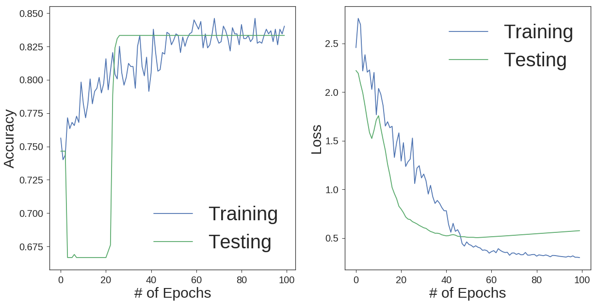
As you can see, we got the classification accuracy of 83% using a neural network. This accuracy would be even better if we had enough training data to train the network better. Then we could employ more hidden layers.
Conclusions:
As shown, it is important to explore the nature of the data set. It is not possible unless we apply different methods on the data. The conclusion that can be drawn is that deep neural networks are the best methods for multi label classification problems. Most of the machine learning algorithms are designed to solve binary (2 class) problems. The only problem with neural networks is the amount of the data required to train the network. For small data sets, the chance of overfitting gets higher. That is why, monitoring the loss function for both training and testing data set is compulsory.
References:
[1] Evett, I. W., & Spiehler, E. J. (1987). Rule induction in forensic science. KBS in Goverment, Online Publications, 107-118.
[2] Pedregosa, F., Varoquaux, G., Gramfort, A., Michel, V., Thirion, B., Grisel, O., … & Vanderplas, J. (2011). Scikit-learn: Machine learning in Python. Journal of Machine Learning Research, 12(Oct), 2825-2830.
[3] Google Pictures.